
Breaking down Google's plan to Double AI Compute Every Six Months
A first‑principles teardown of Google’s Hypercomputer—chips, power, networking, memory, and models—and what actually has to be deleted, rebuilt, and scavenged to make the 6‑month doubling curve real.

Google’s AI infrastructure chief, Amin Vahdat, recently told employees that demand for AI services now requires doubling Google’s compute capacity every six months – aiming for a 1,000× increase in 5 years. This goal, presented at a November all-hands meeting, underscores an unprecedented scaling challenge. This rate of Exponential growth, far outpaces the historical 2× every ~24 months of Moore’s Law. A few months ago we wrote an article breaking down the supply chain that goes into manufacturing the TPUs and mapping out the biottlenecks.
This time we take that to the next level. For Google to achieve the impossible, they must take a page out of Elon’s playbook and:
Deconstruct to Physics. Strip the data center of its racks, cables, and vendors. What remains are the only hard limits: the flow of electrons, the speed of photons, and the rejection of heat. If the laws of thermodynamics allow it, it is possible. Everything else is just legacy.
Rebuild to Economics: We calculate the “Idiot Index” of compute. By comparing the spot price of raw energy and silicon wafers to the current market price of inference, we expose a massive pricing disconnect. This gap isn’t value—it is structural inefficiency. Eliminating it is the only way to make the unit economics of a 1,000× scale-up viable.
Mapping the physics of this 1,000× scale-up uncovers distinct opportunities across the value chain. For our readers at Google, we hope you enjoy this independent analysis and welcome any feedback on our assumptions. For data center operators and power developers, this breakdown separates short-term speculation from structural reality, offering a blueprint to align land and energy assets with the liquid-cooled, gigawatt-scale architectures of the future. Finally, for investors, the opportunity extends well beyond the obvious chip names; we aim to highlight the emerging, critical ecosystems—from photonics to thermal management—that must scale alongside the GPU to make this roadmap possible and as always this is not investment advice.
Supply to FPX. Got spare GPUs/compute, liquid‑ready colo, or powered land with interconnect? List it on FPX—the AI infrastructure marketplace for secondary hardware, colocation, and powered land.Table of Contents
1. Silicon: Breaking the 2.5-Year Chip Cycle
Chiplets, SPAD (prefill vs decode), Lego-style TPUs, and how Google shrinks hardware iteration time.
2. Power: Turning Data Centers Into Power Plants
SMRs, geothermal, boneyard turbines, grid arbitrage, and why power must become part of the design, not an input.
3. Networking: From Packet Cops to Virtual Wafers
Optical circuit switching, Google’s Huygens-class time sync, and designing a fabric that behaves like one giant chip.
4. Memory: Surviving the HBM Bottleneck
HBM scarcity, CXL Petabyte Shelves, Zombie tiers, FP4, and architecting around a finite memory supply.
5. Models: When Intelligence Meets Physics
DeepSeek-style sparsity, Titans memory, inference-time reasoning (o1/R1), world models, and the next era of model–infrastructure co-design.
The 6-Month Doubling Mandate: A “Wartime” Mobilization
At Google’s November all-hands, Infrastructure Chief Amin Vahdat did not present a forecast; he issued a mobilization order. His slide on “AI compute demand” laid out a vertical ascent: “Now we must double every 6 months… the next 1,000× in 4–5 years.”
This is not an aspirational target. It is the calculated minimum velocity required to survive.
The cost of missing this target is already visible on Google’s balance sheet. CEO Sundar Pichai frankly admitted that the rollout of Veo, Google’s state-of-the-art video generation model, was throttled not by code, but by physics: “We just couldn’t [give it to more people] because we are at a compute constraint.” The financial impact is immediate—a $155 billion cloud contract backlog sits waiting for the silicon to serve it. In this high-stakes environment, capacity is no longer just infrastructure; it is the ceiling on revenue.
This only works if silicon, data center, networking, DeepMind and power teams behave like one product org, not five silos. The ‘delete the part’ algorithm applies to org charts too.”
The Game Plan: Beyond Brute Force
Vahdat was explicit: “Our job is to build this infrastructure, but not to outspend the competition.” Achieving a 1,000× gain by ~2029 via checkbook capability is mathematically impossible. It requires a fundamental re-architecture of the computing stack.
Google’s strategy has evolved from simple “scaling” to building a unified “AI Hypercomputer.” This approach attacks the problem from four distinct vectors:
This approach attacks the problem from five distinct vectors:
1. Silicon Specialization (The Physics of Time)
Google is ending the era of the monolithic, general-purpose chip. The new TPU v7 “Ironwood” leverages “Active Bridge” chiplets to break the 30-month design cycle, allowing Google to swap compute tiles annually while keeping the I/O base stable. By splitting silicon into Reader Pods (dense compute for prefill) and Writer Pods (dense memory for decode), they align the hardware to the specific physics of the workload, achieving 3× the throughput per watt over generic GPUs.
2. Thermodynamic Coupling (The Physics of Power)
You cannot plug 1,000× more chips into a standard grid. Google is moving from “consuming” power to “coupling” with it. This means bypassing the grid via Nuclear SMRs and Geothermal sources, and using Liquid-to-Liquid cooling to feed TPU waste heat directly into reactor feedwater systems. By deleting the chiller plant and sourcing power behind the meter, they turn the data center into a thermodynamic co-generator rather than a parasitic load.
3. The “Virtual Wafer” Network (The Physics of Bandwidth)
Scaling to 100,000 chips fails if the network is a bottleneck. Google is deploying Optical Circuit Switches (OCS)—mirrors that route light instead of electricity—combined with a Huygens‑class time‑synchronization stack (nanosecond‑grade clock sync that gives every NIC and TPU the same notion of ‘now’)to create a “scheduled” network. By deleting reactive electrical switches and power-gating electronics during compute cycles, they create a fabric that behaves like a single giant chip (a “Virtual Wafer”) spanning the entire campus.
4. Memory Disaggregation (The Physics of Capacity)
HBM is the most expensive real estate on Earth, and it is sold out. Google is breaking the “private backpack” model where memory is trapped on individual chips. Through CXL “Petabyte Shelves” and “Zombie” Tiers (recertified storage), they allow TPUs to borrow capacity instantly from a shared pool. Simultaneously, they are using Synthetic Data to enable FP4 (4-bit) training, effectively quadrupling the capacity of every HBM stack in the fleet without buying new silicon.
5. Model Co-Design (The Physics of Intelligence)
Hardware alone cannot bridge the gap. Learning from the efficiency of DeepSeek and the constraints of physics, Google DeepMind is rewriting the model architecture itself. This includes adopting Multi-Head Latent Attention (MLA) to slash memory usage, Titans architecture for long-term neural memory (replacing context window bloat), and System 2 “Cortex” logic that trades time for parameters. The goal is to escape the “Transformer Monoculture” and build models that inherently require fewer joules per thought.
FPX: The AI Infrastructure Marketplace. We run a secondary hardware marketplace (recertified accelerators, DRAM, SSD/HDD), place it into liquid‑ready colocation, and bundle powered land with interconnect so you can scale now. When supply chains stall, we get creative and fix bottlenecks.We’ll start with the part that looks the most familiar from the outside — the chips — and then follow the constraints outward into power, networks, memory, and finally the models themselves.
1) Silicon: Matching Hardware to the Speed of Intelligence
1) Breaking It Down to the Physical Constraints
If you ignore the branding and SKUs, Google’s AI hypercomputer is bounded by four hard things:
Time – how fast you can change silicon.
Calculation – how much energy each useful operation burns.
Bandwidth and distance – how far bits have to travel, and through what medium.
Intelligence – how many bits you really need to represent the world and keep state.
TPUs, Axion, Titanium, Apollo, Firefly, SparseCore – these are not random product names; they’re successive attempts to align the machine with those four constraints. The question isn’t “are they doing enough?” but “what else can be deleted?”
The Physics of Time: silicon moves in years, models move in months
The first hard limit is temporal. Leading‑edge chips still move on a roughly 2–3‑year design/fab cycle. Large models, attention mechanisms, agent architectures and serving patterns are turning over in 6–12 months. That mismatch is why chips end up bloated: because you can’t know exactly what Gemini‑4 or some agentic successor will look like, you overbuild “just in case.”
The way out, from a physics point of view, is to stop treating a TPU as a single static object. You freeze the “slow physics” parts and you spin the “fast physics” parts.
Slow physics: I/O PHYs, high‑speed SerDes, HBM interfaces, power delivery, security islands – analog, timing‑critical, painful to re‑verify. Fast physics: systolic arrays, sparsity engines, precision formats, routing logic – the math and the dataflow.
The Active Bridge / Lego Pod metaphor is useful here. Instead of one mega‑die, you build:
a long‑lived base tile for I/O + HBM
one or more Math Tiles that you can respin yearly
and a bridge that makes them behave like one chip
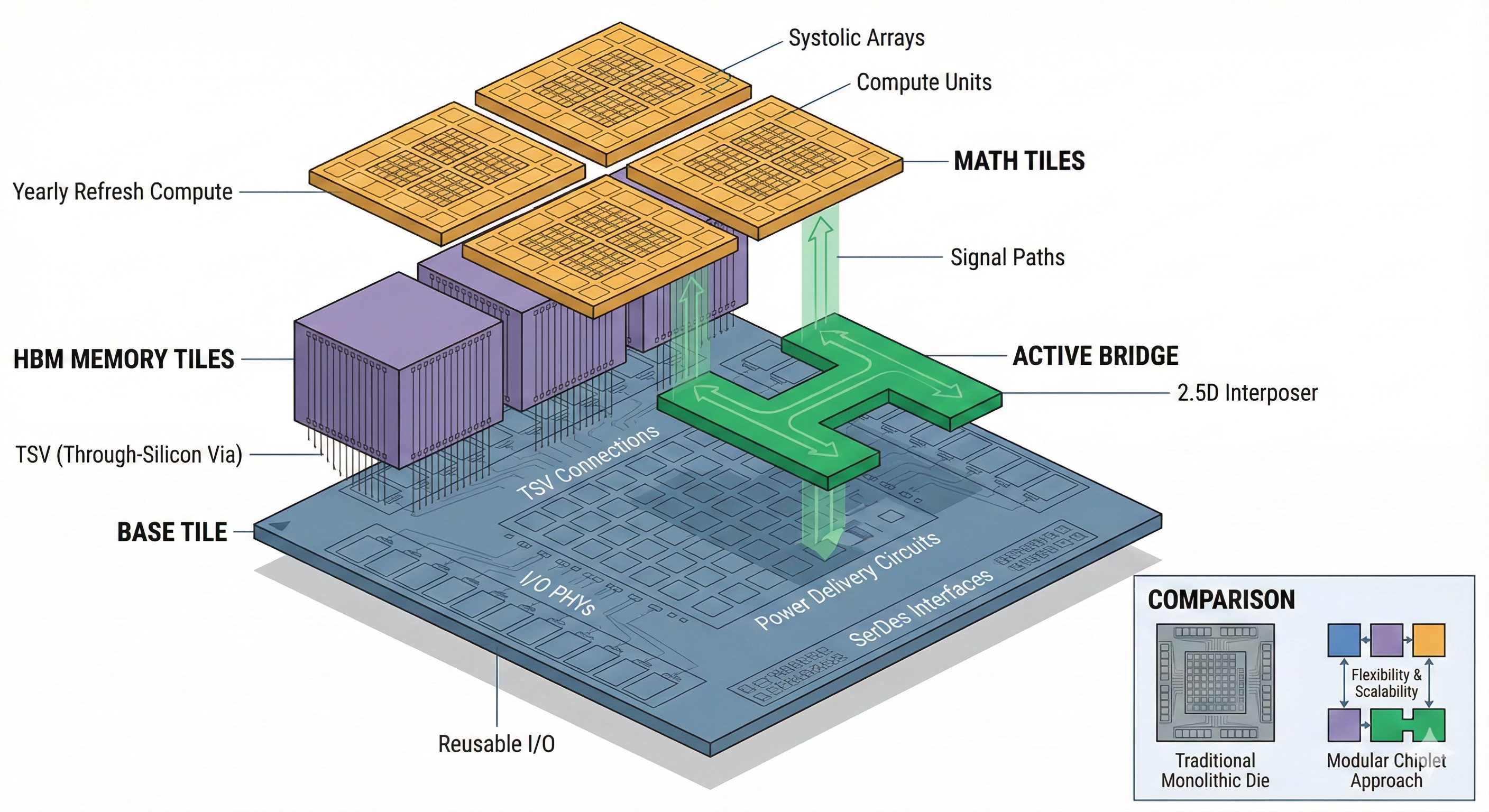
Once you have that, the “chip” becomes a configuration problem. A training or prefill‑heavy pod might be four Math Tiles and two HBM tiles bolted to a bridge. A decode‑heavy pod might be one Math Tile and eight HBM tiles. Same tiles, same manufacturing stack, completely different physics profile.
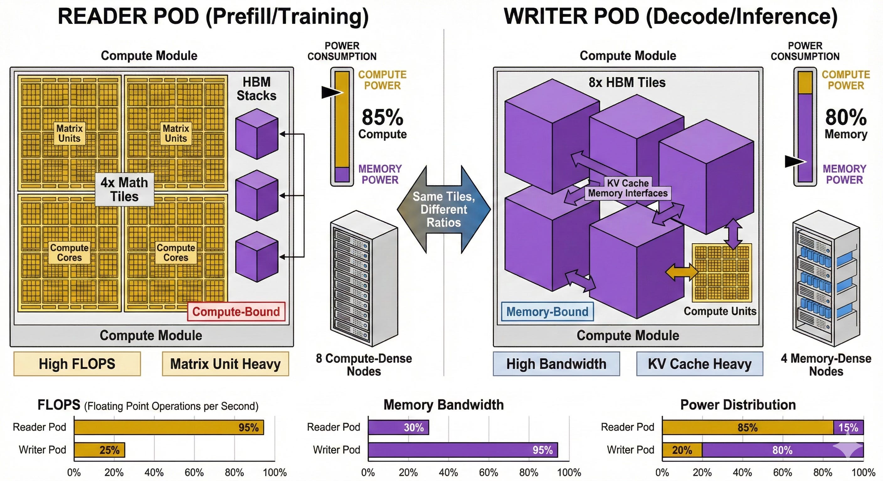
SPAD —> Specialized Prefill And Decode, is the physics-aligned insight that an LLM isn’t one workload, but two. Prefill is compute-bound: square matrix multiplies that want wall-to-wall MXUs and dense FLOPs. Decode is memory-bound: KV lookups and skinny matmuls that sit idle unless you feed them bandwidth and HBM. Traditional GPUs try to be “ambidextrous” and serve both phases, which means they’re great at neither. SPAD flips that: build one kind of silicon for prefill (Readers), another for decode (Writers), and wire the fabric so each token is handled by the hardware whose physics actually fits it.
Ironwood is already a step in this direction: it’s explicitly an inference‑first TPU with more aggressive perf/W, heavy matrix units, and the expectation that it will be replaced more rapidly than the underlying data center fabric. SPAD‑style “Reader/Writer” specialization is just the logical endpoint of that trend.
Time isn’t just in the design tools; it’s also in the logistics. The speed of light is not your enemy here; the speed of FedEx is. That’s why Google’s new hardware hub in Taipei matters: it collapses the loop between TSMC, packaging, and Google’s own engineers. The extreme version of this is a “zero‑mile fab”: a Google‑only test lab bolted onto the fab and packaging line, where wafers can be probed by Google’s own validation rigs hours after they come out of the ovens, not weeks later when they’ve cleared customs and been shipped across the Pacific. In a war of exponential curves, shrinking the iteration loop from three weeks to three hours is its own kind of physics.
The Physics of Calculation: prefill vs decode, and Ironwood as SPAD v0
Next constraint: the cost of math.
LLMs have two very different phases from a physics viewpoint:
Prefill – ingest the prompt. Big, square matrix multiplies; high arithmetic intensity; compute‑bound.
Decode – generate tokens. KV cache lookups in HBM; skinny matmuls per step; memory‑bound.
Classic GPUs and early accelerators are ambidextrous by design: one chip is supposed to handle training, prefill, decode, recsys, you name it. That means in prefill you’re starved on FLOPs, and in decode those FLOPs mostly sit idle waiting for memory.
Google already did the optimization Step‑1 once here. TPUs deleted a lot of general‑purpose junk – huge caches, branch predictors, wide scalar ALUs – and rebuilt around systolic arrays and scratchpads. They added SparseCore as a tiny on‑die dataflow engine for embeddings and routing, so the main arrays don’t have to waste cycles on those patterns. From a physics perspective that’s: delete speculative hardware, push the intelligence into the compiler (XLA), and only put transistors where math actually happens.
SPAD is the next delete: stop pretending prefill and decode belong on the same die. You want a Reader that is basically wall‑to‑wall matrix units with just enough memory to keep them full, and a Writer that is mainly HBM capacity and bandwidth with little compute sprinkled near each stack.
Ironwood already leans heavily into the “Reader” role – an inference‑first TPU with beefed‑up systolic arrays and perf/W tuned for serving. The architectural ideal we’re talking about is just making that split explicit at the package level. With chiplets, you don’t need separate product lines; you vary the ratio of Math Tiles to HBM tiles per pod. One configuration looks like a prefill cannon; another looks like a KV cache farm.
And then there’s routing. Not every token needs to see every layer. DeepMind’s mixture‑of‑experts and mixture‑of‑depths work is exactly about that: easy tokens exit early; hard ones go deep. SparseCore is the right place to embody that physically. Instead of quietly sitting in the corner accelerating embeddings, it becomes a brainstem: a small organ that decides which tokens go where and which never touch the big MXUs at all. Every token that early‑exits is a pile of FLOPs and joules you never spend.
The Physics of Bandwidth and Distance: from packet cops to a virtual wafer
Bandwidth isn’t really about “how many terabits” your spec sheet says. It’s about how far bits travel, what medium they travel through, and how much thinking the network has to do about them.
Electrons in copper are slow, hot, and lossy. Every long trace and every SerDes hop costs you energy per bit and nanoseconds of latency. Packet switches exist to make per‑packet decisions because the network was designed assuming traffic is random. That’s why a big Broadcom switch chip happily burns half a kilowatt just parsing headers and juggling queues. It’s all reactive.
AI workloads aren’t random. Training collectives are literally graphs; we know the all‑reduce steps before we launch the job. Even inference isn’t truly chaotic once continuous batching gets involved. Systems like vLLM take a swarm of incoming user prompts, buffer them for a few milliseconds, and pack them into dense, regular batches. From the network’s point of view, it suddenly looks a lot like training: large, predictable bursts of tensors.
This is where Google’s optics are quietly radical. Apollo replaces a whole spine layer of packet switches with optical circuit switches – MEMS mirrors and glass. The mirrors don’t make decisions; they just sit at whatever angle the control plane told them to assume. Combine that with Huygens‑class time‑synchronization stack sync (NICs all marching in nanosecond lockstep) and AI‑first NICs, and you get a fabric that can be scheduled rather than policed.
In that world, you don’t route packets, you timetable bursts. The compiler/runtime knows when gradients are going to fly or when a batch of prompts is going to be scattered; it can instruct the OCS to re‑wire the graph a few milliseconds in advance. During compute phases, the links can go mostly dark or be repurposed for checkpointing. During comm phases, all links are hot, and no one is stuck in a buffer because collisions simply aren’t allowed by construction.
This is where the economic bridge starts to show through. The Idiot Index of a standard switch is high because it creates heat to make decisions. Apollo creates almost no heat and makes no decisions. It just follows orders. By moving the “intelligence” (routing) to the compiler and the “labor” (switching) to mirrors, Google has effectively driven the marginal cost of moving a byte toward zero. The optical core and the fiber don’t care if endpoints are speaking 100 G, 400 G, or 1.6 T – they will happily reflect whatever hits them. You stop ripping out the nervous system every time a new chip doubles its SerDes rate; you just plug faster lasers into the same glass.
From a physics standpoint, that’s the closest you can get to a virtual wafer: tens of thousands of chips and a couple of petabytes of HBM talking to each other as if they were a single coherent device, because most of the “distance” is traveled at the speed of light in a passive medium.
The Physics of Intelligence: synthetic data arbitrage and stateful silicon
The last constraint isn’t in the metal; it’s in the bits we push through it.
HBM is already the tightest resource in the system: capacity, bandwidth, and energy per access all bite. One lever is precision. Hardware has raced ahead to support 8‑bit and even 4‑bit floating‑point formats for both training and inference. The catch is that the internet is a mess. Training at 4 bits on raw, noisy web text is like doing surgery with oven mitts on: technically possible, but you wouldn’t trust the result.
The sensible first‑principles play is what you could call synthetic data arbitrage. Instead of trying to make ever more heroic quantization schemes, you change the data so low precision is actually safe. Gemini‑class models are already good enough to rewrite ugly, inconsistent web pages into structured, textbook‑like knowledge. If you use them to clean, summarize, and normalize your pretraining corpus, you can manufacture a dataset with:
fewer pathological outliers
more consistent distributions
less adversarial garbage
That’s a corpus where 4‑bit statistics make more sense. If you then design your training curricula and architectures around that reality, you can push more of the model into FP4/INT4 without collapse. Every bit you delete halves your memory needs for that part of the network. That’s not free – it costs cycles upfront to synthesize the data – but it’s a capital trade you make once for a fleet‑wide gain.
The 4‑Bit Direction: Using Fewer Bits, More Often
Today, most frontier models still train in BF16 or FP8 and only use 4‑bit formats (FP4/NF4) for parts of the stack or for inference. Pushing everything to 4 bits overnight would blow up optimization. But the direction of travel is clear: every tensor that can safely drop from 16‑bit → 8‑bit → 4‑bit frees scarce HBM capacity and bandwidth. NVIDIA’s Blackwell and the next TPU generations are being built with native FP4 support for exactly this reason: they expect a growing fraction of weights, KV caches, and optimizer states to live at 4 bits, at least during inference and later stages of training. Google doesn’t need “full FP4 training” on day one to win — it needs a roadmap that steadily expands the share of the model that can tolerate 4‑bit without collapsing.
Synthetic Data as a Low‑Bit Enabler
Raw web text is numerically ugly: outliers, adversarial junk, wild distribution shifts. That’s exactly what makes extreme quantization brittle. The real value of Gemini‑class synthetic data is not just “more tokens,” it’s better‑conditioned tokens. If Google uses its strongest models to rewrite the internet into textbook‑like corpora — consistent style, fewer outliers, clearer supervision signals — it can safely push more of the training and inference pipeline into FP8 and FP4. Clean data doesn’t magically make 4‑bit trivial, but it widens the stability margin for quantization‑aware training and mixed‑precision regimes. In practice, that means every year a larger slice of the model can drop to 4‑bit, turning the same fixed HBM budget into more usable parameters and longer contexts.
There’s a second “intelligence” constraint emerging that’s newer: state. Google’s launch of agent‑first tooling like Antigravity changes the workload from “stateless two‑second chats” to “stateful four‑hour work sessions.” Current TPUs are basically amnesiacs: they serve a request, flush most of the interesting state from on‑chip memory, and load fresh context from HBM next time. That’s fine for single prompts; it’s brutal for long‑lived agents that need a large, evolving working set.
The physics fix there is different: you need stateful silicon. Think of a “Cortex Tile”: a chiplet that is mostly SRAM – static RAM on‑die – rather than HBM. SRAM is expensive in area but ~100× faster and lower‑energy per access than DRAM. You don’t deploy it everywhere; you buy a specific rack of Cortex TPUs that exist primarily to hold agent state in SRAM for hours at a time, while more generic compute tiles rotate through to do the heavy lifting. Instead of constantly re‑hydrating context from cold storage and HBM, your agents live in a warm, electrically‑near memory pool.
From a physics perspective, that’s just another specialization: HBM tiles for bulk parameters, SRAM tiles for hot, agentic working sets. From an economic perspective, you’re reserving your most exotic silicon for the most valuable, long‑running workloads rather than wasting fleet‑wide capacity on state that 95% of users don’t need.
Rebuilding to Economics: lowering the Idiot Index
Once you’ve stripped everything down to physics, you can start putting the dollars and watts back in and ask how dumb the current setup really is. That’s where the “Idiot Index” is useful: it’s the ratio between what you pay per token today and what you would pay if you were perfectly aligned with energy and wafer costs.
Chiplets and Lego Pods are a direct attack on that index. By splitting TPUs into long‑lived plumbing and fast‑moving math, Google reduces both capital risk and wasted silicon. You’re no longer betting billions on a single mega‑die that may or may not age well. You’re betting on an I/O + HBM base that you’ll reuse across multiple math generations, and much smaller Math Tiles you can afford to be aggressive with. When models change, you don’t throw away your entire design; you respin the piece that enforces the new math.
Free the fast silicon. FPX backfills everything that isn’t MXU‑hot: Shelf Bricks (CXL DRAM pools) and Checkpoint/Context Pods (recertified SSD/HDD). Keep HBM for prefill and math—push KV, logs, and checkpoints into cheaper tiers.
SPAD‑style specialization does the same thing in “compute space.” An ambidextrous chip spends a lot of its life as dead weight: training logic sitting idle during inference, or big MXUs sulking during decode. A Reader/Writer split implemented via tile ratios means each pod spends more of its energy doing the kind of work it’s physically good at. Even if the wafer cost never budges, the tokens per watt and tokens per dollar go up because you’ve stopped paying for transistors on vacation.
Axion and Titanium are the economic reflection of what TPUs did architecturally. Instead of paying Intel or AMD for huge, general‑purpose CPUs that spend their lives shuttling buffers and handling IRQs, Google runs its own Arm host and offloads networking and storage into dedicated controllers. The host becomes a thin control plane, not the star of the show. That’s vendor margin erased from the BOM and host power reclaimed for accelerators. The physics is simple – don’t burn energy on work the TPU or NIC can do more efficiently – and so are the economics.
The networking story is where the Idiot Index really collapses. Traditional AI clusters are on a treadmill: every bump in line‑rate forces a new generation of copper and switch ASICs, plus the labor to rip and replace them. You are, in effect, paying constantly to move heat around inside boxes that make decisions. Apollo flips that: the core is glass and mirrors that never learn, never think, never age out of a spec. You move “intelligence” up into XLA, Pathways and the batcher, and let mirrors be stupid. The result is that the marginal cost of moving another byte across the fabric is dominated by endpoint energy, not by the spine. The network becomes like a 400 V bus bar or a concrete slab: a long‑lived asset you amortize over many chip generations.
Synthetic data arbitrage and low‑bit formats attack the two most expensive invisible line items in an AI box: HBM and joules per DRAM access. If a year of work on data cleaning and training recipes lets you reliably run large swaths of your models at 4 bits instead of 16, you effectively double your usable capacity and cut memory opex per token in half. The work you did once in the data pipeline compounds across every pod you deploy.
The honest way to think about FP4 is not ‘we will train everything in 4‑bit next year,’ but ‘every year, another slice of the model safely moves to 4‑bit.’ The winner is the lab that moves the largest share of its workload down the precision ladder without losing quality.
Stateful silicon for agents looks expensive on paper – SRAM‑heavy tiles are not cheap – but it is the right kind of expense: tightly targeted and physics‑aligned. If you know that a small fraction of sessions (say, a trading agent, a code‑review copilot, an operations “AI SRE”) dominate value and have long, rich state, it is economically saner to buy a few racks of Cortex‑style tiles to house those brains than to force the entire fleet to reload their world from cold storage on every call.
Zoom out, and a pattern emerges. The moves that look “hardware‑nerdy” in isolation – chiplets and active bridges, SPAD‑like pods, SparseCore routing, Apollo optics, Huygens‑style time‑sync schedules , Axion/Titanium hosts, synthetic low‑bit data, SRAM‑heavy cortex racks – are all the same move repeated: align the machine with the underlying physics so ruthlessly that anything wasteful stands out as an accounting error. Once you do that, the economics start to bend. The Idiot Index comes down, and Amin’s “1,000× in roughly five years at similar cost and power” stops sounding like bravado and starts looking like a reasonable target for a company willing to delete everything that doesn’t serve the electrons, the photons, and the heat.
What This Means for Data Center Operators
How SPAD, virtual wafers, and task-specific silicon reshape facilities
As Google leans into physics-aligned architectures—splitting prefill and decode workloads, designing SPAD-style Reader/Writer pods, and treating thousands of TPUs as a single “virtual wafer”—the data center stops being a generic compute warehouse and becomes a set of specialized organs. Training and prefill jobs want remote, high-density campuses built for liquid cooling and massive optical backbones. Decode and real-time inference want smaller metro sites sitting close to IXPs, with more HBM and network bandwidth than raw compute. Long-lived agent workloads introduce a third category: stateful halls with SRAM-heavy “cortex” racks that hold multi-hour context in fast memory while compute tiles rotate around them. Operators who recognize this shift early can pre-position themselves by designing three distinct facility types—compute factories, metro inference hubs, and state hubs—each optimized for the physics of its workload and compatible with chiplet-style TPUs, optical fabrics, and high rack densities. Doing so makes the operator a drop-in extension of Google’s hypercomputer rather than a retrofit compromise.
FPX for Operators. Bring liquid‑ready, high‑density suites and fiber‑rich halls; we place secondary hardware and memory shelves to create SPAD‑aligned Reader/Writer/Cortex zones. New revenue from existing space.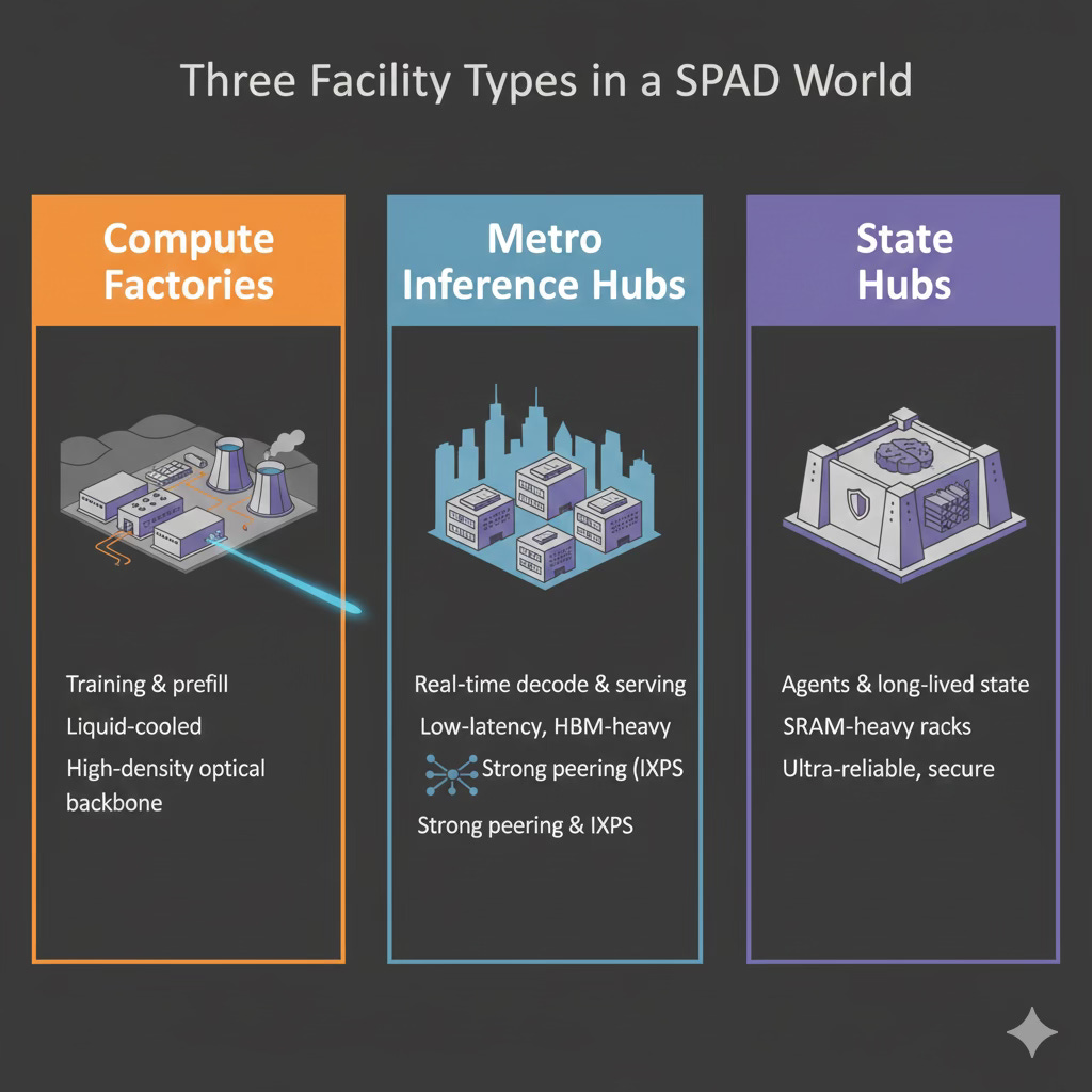
How Operators Gain an Edge (and How to Prepare Now)
Operators who prepare for this split win by becoming TPU-ready before TPU demand arrives. That means:
Adopting liquid cooling, 400 V busways, and fiber-dense hall design as defaults—not upgrades.
Building white-space that can host Reader/Writer pod ratios (compute-heavy vs. HBM-heavy racks).
Designing campuses around long-lived optics and power infrastructure, not around switch ASIC refresh cycles.
Marketing real estate not as “capacity,” but as specialized tiles Google or any hyperscaler can snap into their virtual wafer.
Being early here turns the operator into an AI-grade infrastructure partner, not just a landlord—making them relevant for multi-cycle deployments instead of single-generation GPU scrambles.
Fabric‑ready shells sell. List metro inference suites, memory/shelf rows, and training‑grade halls on FPX. We match your envelope (space + fiber + MW) to live AI demand.What This Means for Investors
How to price powered land, colo shells, and optical-ready campuses in a SPAD world
When prefill, decode, and agent workloads split into different physical requirements, not all megawatts or square feet are equal anymore. The winning assets will be those aligned with the physics: large powered land near cheap generation for prefill/training pods; metro-edge shells with excellent peering for decode; and ultra-reliable, ultra-secure campuses that can house stateful SRAM-heavy “cortex” racks. Investors should understand that the value migrates from servers to the envelope—the power, fiber, cooling, and zoning that support a decade of TPU evolution. Facilities built around optical fabrics (like Google’s Apollo-style architectures) become long-lived utilities, while racks and GPU generations turn over rapidly. This creates asymmetric upside for owners of “future-proof” land and infrastructure.
How Investors Gain an Edge (and What to Do Now)
Prioritize powered land near hydro, nuclear, or major substations—perfect for prefill/training factories.
Accumulate metro-edge colos with rich peering for decode and agent workloads (these become the new latency-critical frontier).
Back operators modernizing to AI-grade spec: liquid cooling, 50–80 kW racks, optical-first design, 400 V distribution.
Favor long-lived infrastructure plays (glass, power, entitlements) over single-generation hardware exposure.
The thesis is simple: Google’s architectural shift creates a structural demand frontier for AI-ready land, optics-ready shells, and specialized facilities. Investors who position ahead of this curve aren’t just riding the GPU boom—they’re buying the foundational real estate of the next compute era.
Own stranded assets? FPX packages them into AI‑grade supply. FPX converts retired accelerators, media, brownfield MWs, and shells into standardized SKUs tenants actually buy. If you control the atoms, we’ll clear the path to AI demand.
2) Power & Thermodynamics: When Energy Becomes the Hard Limit
Power is the bottleneck that doesn’t care how clever your model is. At today’s ~30,900 TWh of annual electricity use, the world runs at an average of about 3.5 TW. If the industry truly built out ~300 GW of new AI datacenter load every year, we’d blow past all current global generation in just over a decade. That’s before EVs, heat pumps, or industrial electrification even show up. You don’t solve that by “plugging in more TPUs.” The physics is brutal: you take high‑grade electrical energy, turn it into low‑grade heat in the chip, then burn more electricity on chillers and pumps to throw that heat into the air. In thermodynamics, the portion of energy that can actually do useful work is called exergy; current AI infrastructure wastes a huge amount of it. To get 1,000× more compute without 1,000× more emissions and blackouts, you have to stop treating power and cooling as line items, and start treating them as a coupled thermodynamic system you can engineer.
Phase 1 – Deconstruct to Physics: Energy Density & Heat Rejection
At the physical level, every watt that goes into a TPU comes out as heat. A typical hyperscale data center still follows the same pattern: the grid feeds a substation; the substation feeds power distribution units (PDUs); PDUs feed racks; racks dump heat into air or water; then a chiller plant spends another ~20–40% of the IT load’s power turning that hot water back into cold water. The industry uses a metric called PUE (Power Usage Effectiveness: total facility power divided by IT power). A “good” PUE today is ~1.2. From a physics lens, that’s still an Idiot Index: you built a second power plant whose only job is to undo what the first one did.
That waste shows up inside the chips too. Because of process variation (random manufacturing differences between dies), some TPUs are “golden” (low‑leakage, high‑yield), others are dogs. The safe thing is to set voltage and frequency for the worst chip in the fleet—say 0.8–0.85 V—and run every part there. Most of your silicon is over‑volted relative to its actual physical limit, burning extra dynamic power just so the worst 1% doesn’t glitch. You’re paying for randomness in the fab as if it were a law of nature.
The network stack leaks energy in the same way. Even when no useful packets are flowing, lasers, SerDes (serializer/deserializers that encode bits onto high‑speed links), and DSPs sit there sipping watts to stay synchronized and ready. Yet AI traffic is not random. Training jobs “breathe”—hundreds of milliseconds of pure compute, then brief all‑reduce bursts to exchange gradients. Inference stops looking like Brownian motion once you add continuous batching: the serving stack buffers user queries for a few milliseconds and fires them as dense, predictable bursts instead of tiny dribbles. The fabric sees trains, not cars.
On top of that, the grid itself is slow and lumpy. Building a new 500 MW substation and its transmission lines is a 5–10‑year permitting fight in most jurisdictions. Nuclear small modular reactors (SMRs) like Kairos’s Hermes‑2 will bring Google tens of megawatts by around 2030 and up to ~500 MW by 2035—but that’s a 2030s answer, not a 2027 patch. Even geothermal, where Google and Fervo’s “Project Red” is already delivering 24/7 carbon‑free power in Nevada, scales in hundreds of megawatts, not gigawatts overnight. Put differently: the natural timescale of the grid is years; the AI build‑out is moving in quarters. That mismatch is the true physical constraint.
FPX Power Envelopes: 50–500 MW you can actually use.
We package powered land + interconnects + permits—often with temporary generation (refurb aero‑turbines), shared industrial cooling, or geothermal tie‑ins—so your AI campus lands on a realistic timeline. We also broker interconnection queue positions and substation piggybacks where industrial feeders are under‑utilized. Pair that with training‑as‑flexible load and you get lower blended power costs and faster approvals.
Phase 2 – Rebuild to Economics: From Consumption to Coupling
Once you admit the grid’s timescales and thermodynamics, the first principle move is clear: stop “consuming” power in whatever form the grid hands you; couple your compute directly to the sources, pipes, and waste streams where physics is already on your side. The job is to turn power from a bill into a design variable.
2.1 Co‑locate with the atoms: nuclear, geothermal, and thermal reuse
Google’s 500 MW deal with Kairos Power is usually framed as “buying green electrons,” but the deeper move is thermal integration. SMRs are essentially steady high‑temperature heat engines: they already have massive cooling loops and “ultimate heat sinks” designed to dump gigawatts of heat into rivers or towers. If you stick a data center right next to that, you don’t need a fully separate chiller plant. You can drive absorption chillers—devices that use heat, not electricity, to make cold water—off the reactor’s waste heat, and share cooling towers and water infrastructure instead of duplicating them.
Push the coupling one step further and you get what you might call the liquid‑to‑liquid loop. Nuclear steam cycles spend a lot of energy pre‑heating feedwater from ambient to near boiling before it enters the reactor. TPU coolant loops run at 50–70 °C. Instead of cooling that back to ambient and throwing it away, you can use it as a pre‑heater for the plant’s feedwater. The AI farm becomes a cogeneration unit: its “waste” heat raises the temperature of the water that will be boiled by the reactor anyway. You haven’t literally violated conservation of energy—there’s still an ultimate heat sink somewhere—but you’ve effectively shrunk the stand‑alone cooling plant on the data‑center side and improved the power plant’s thermal efficiency on the other. One set of pipes does double duty.
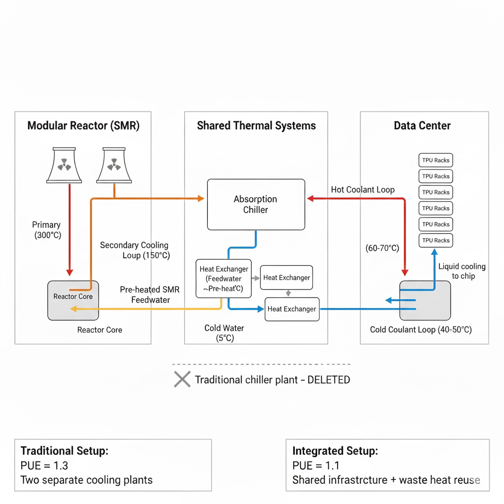
Because SMRs take the rest of the decade to arrive, the 2020s bridge is geothermal. Google’s early work with Fervo in Nevada and follow‑on clean‑transition tariffs show how enhanced geothermal systems (deep drilled wells that use oil‑and‑gas‑style techniques to reach hot rock) provide 24/7 carbon‑free power today. From an engineering perspective, an EGS plant looks a lot like a data center already: closed‑loop pipes, big pumps, and heat exchangers. Putting AI pods on the same site lets you share those loops, run higher rack densities (because you have process‑grade cooling anyway), and guarantee firm power without waiting for a new reactor license.
The same logic extends to other industrial sites. LNG terminals and some chemical plants have excess cold (they’re literally boiling cold liquids back into gas); refineries, steel mills, and paper plants have excess low‑grade heat. Data centers can be the thermal sponge in either direction:
Next to “cold” plants, direct‑to‑chip loops can be cooled via liquid‑to‑liquid exchangers, shrinking or deleting most of the data center’s own chiller plant.
Next to “hot” plants or SMRs, AI exhaust heat can be sold as process heat or feedwater pre‑heat, lowering both sides’ effective energy cost.
In all cases you’re using the same joule twice—once for computation, once for heat work—instead of paying for two separate energy systems.
2.2 Bootstrap power fast: boneyard turbines, zombie peakers, and flared gas
Nuclear and geothermal are great, but they are slow. Google’s 1,000× target is not going to wait for every SMR to clear the NRC. So the next class of moves is ugly but fast: reuse metal that already exists.
One obvious pool is retired aircraft engines. Widebody fleets are being scrapped faster than their turbofans wear out. Gas‑turbine specialists already convert engines like GE’s CF6 into stationary 40–50 MW peaking units; the physics is done, the engines are sitting in boneyards, and the lead times are a fraction of a new utility‑scale turbine. The gating factor becomes local air permits and politics, not global turbine backlogs. The build fast; iterate later , move here is: don’t sit in the four‑year queue for brand‑new gas turbines; buy the boneyard, refurbish, and drop 50 MW “jet‑gens” behind the meter at AI campuses. FPX’s role is obvious—source and procure those used engines, match them to brownfield sites, and coordinate OEM‑backed refurb programs so the reliability looks like aviation, not DIY.
The same idea applies at plant scale. There are “zombie” peaker plants all over the world: gas and even coal facilities that still have 250–500 MW substations, cooling water rights, and industrial zoning, but can’t make money in normal capacity markets. Their wires and permits are worth more than their boilers. Rolling them up into an “AI power fund” lets you buy those interconnects and switchyards at distressed prices, then repower the generation (with gas‑only, high‑efficiency turbines, used aero engines, or eventually SMRs) while you drop modular TPU pods on the existing pads. You’re not building new substations; you’re compressing more compute into substations that somebody else already paid for.
Then there’s the dirty bridge: flared gas. In North Dakota and West Texas, operators literally burn surplus natural gas at the wellhead because there’s no pipeline capacity; 100% of that chemical energy turns into heat and light in the sky. Thermodynamically, the Idiot Index of flaring is infinite. If you park containerized AI pods and small turbines on the pad, you’re still emitting CO₂, but you are at least getting useful compute out of energy that was otherwise pure waste. This is not the end state—you eventually want those sites replaced by geothermal or nuclear—but as a bridge, “flare‑to‑compute” is strictly less bad than flare‑to‑nothing, especially if it’s paired with a clear sunset plan and offsets.
None of these moves are easy. Zombie peakers and aero‑turbines run into air permits and local resistance; flare‑to‑compute offends ESG purists even when it’s thermodynamically better than flaring; SMRs fight national politics. But physics doesn’t care about press releases, and neither does a 300 GW/year build‑out.
2.3 Arbitrage the grid itself: queues, substations, and FPX‑style power envelopes
A subtler bottleneck is that a lot of power is stuck in paperwork. Interconnection queues in the U.S. and Europe are clogged with solar farms, hydrogen projects, crypto mines, and generic industrial loads that may never be built. Brownfield factories sit under 100 MW feeders while their actual load shrank to 20 MW years ago. From a physics view, those are stranded rights to move electrons, not just stranded assets.
This is where an power exchange becomes interesting. Instead of only trading compute capacity, the market starts trading grid positions and latent substation headroom. A stalled 80 MW solar project in Ohio might be three years from financing; its developer sits on a valuable queue slot but no capital. FPX can broker a lease or sale of that queue position to Google (or any AI player), who drops in containerized training pods for 5–7 years while their own permanent campus is being built. When the solar farm is finally ready, the AI pods move on but the substation upgrades and legal work remain. Similarly, FPX can identify industrial sites with under‑used feeders, assemble “substation piggyback” deals where an AI tenant shares capacity and time‑slices with the host, and package those as ready‑to‑go 50–200 MW chunks.
This is exactly the direction Meta is moving with Atem Energy, its new subsidiary that has applied for authority to trade wholesale power and capacity. Meta’s play is clear: become its own power trader so it can arbitrage prices and secure flexible supply for 2 GW‑class AI campuses, rather than relying on utilities alone. That’s a signal that hyperscalers no longer see electricity as a simple pass‑through; they’re willing to carry trading risk on their own balance sheets if it buys them certainty. FPX doesn’t have a formal exchange product today, but it already does the hard part: sourcing and procuring used power infrastructure—generators, turbines, substations, and distressed datacenter shells. The natural next step is to surface those as standardized “power envelopes”: brownfield land + interconnect + sometimes temporary generation, sold as bundles AI companies can simply plug into.
FPX “Grid Desk.” We surface queue slots, latent substation headroom, and brownfield feeders as tradable envelopes. You bring the pods; we bring the electrons and paperwork you can stand on.2.4 Make AI a grid asset, not just a load
Not all power solutions are on the supply side. AI’s weird superpower is that training is elastic: you care that the model is done this week, not that every gradient step ran at exactly 2:34 p.m. In grid language, training is a “flexible load.”
If Google exposes that flexibility to the grid operator, AI becomes a kind of virtual power plant. When there’s too much solar at noon, Borg and the batcher spin up training jobs and prefill‑heavy workloads; when the sun sets and the grid tightens, they checkpoint and throttle down, freeing hundreds of megawatts without any human noticing. Structured as demand‑response or frequency‑regulation products, that flexibility is something utilities pay for. The net effect is lowering Google’s average power price and making regulators eager to approve new AI campuses because they come with built‑in controllability instead of just more peak demand.
At the micro level, the same principle applies on die. Google already has tools to hunt “mercurial cores” and silent data corruption; that telemetry can be reused to create software‑defined voltage and frequency per chip. Golden TPUs can be safely undervolted toward their individual physics limits, shaving 10–20% dynamic power; weaker dies can be fenced to low‑priority, low‑clock jobs. Across 100,000 chips, that’s a free power plant’s worth of savings with no new hardware—just a willingness to treat V/f as a software knob instead of a fixed spec.
And don’t forget the network. Optical circuit switches (OCS) built with MEMS mirrors typically reconfigure in milliseconds, not microseconds—far too slow for per‑packet routing, but perfectly fine for the 50–300 ms “breaths” of an AI job once continuous batching has packed the workload into trains. Time‑sync schedules means the NICs know exactly when each breath arrives; the mirrors can rewire a few tens of milliseconds beforehand. In that world, you can power‑gate the hungry SerDes and DSP electronics for most of the cycle, keeping lasers in low‑power idle or burst‑mode, brightening only when the schedule says “burst now.” Across millions of links, turning off the electronics during the 70–80% of time when nothing useful is flowing is another huge chunk of “invisible” power reclaimed.
2.5 Go where the photons are: training in space, inference on Earth
Finally, there’s the move that feels like sci‑fi but is already on the roadmap: space‑based compute. Google’s Project Suncatcher is a research moonshot to put TPUs on solar‑powered satellites in dawn–dusk orbits, talking over free‑space optical links. In orbit you get near‑continuous solar, several times the energy yield per square meter of panel compared with many locations on Earth, and a 3 K cosmic background as your heat sink. Latency and radiation make it impractical for user‑facing inference, but for long‑running training loops it’s plausible on a 10‑year horizon if Starship‑class launch really delivers hundreds of tons to orbit cheaply.
The physics split is neat: inference stays on Earth, close to users, data, and regulation; training migrates to wherever energy density and heat rejection are best—eventually that might be space. Google plans to launch small Suncatcher prototypes around 2027 to test TPUs in radiation and optical cross‑links; any commercial version is likely a mid‑2030s story at best. But the direction is consistent with everything else: follow the photons and the cooling, not the legacy substations.
Pulling it together
All of these moves—nuclear co‑location, geothermal bridges, boneyard turbines, zombie peaker roll‑ups, flared‑gas pods, queue and substation arbitrage, industrial symbiosis, AI‑as‑flexible‑load, orbital training constellations—are variations on the same theme: stop treating power as an exogenous constraint and start designing the AI stack around the physics of energy.
For Google, that means Amin Vahdat’s 1,000× target can’t just be a story about better TPUs and smarter compilers. It has to be a story about where the atoms, pipes, queues, and photons are—and about partnering with firms like FPX that are willing to do the unglamorous work of scavenging turbines, brownfield substations, interconnect slots, and stranded wells. For FPX, it’s the opportunity to position itself as the Atem of infrastructure: not a power trader, but the specialist that finds, assembles, and procures the weird, messy assets—old plants, queue positions, used generators, and eventually orbital power slots—that will quietly decide who actually gets to build the next 10 GW of AI.
For investors
the power section is basically a filter for what will actually be scarce and valuable over the next decade. It says: stop thinking in terms of “more data centers” and start thinking in terms of where exergy lives. The assets that benefit from 1,000× AI aren’t generic shells; they’re powered dirt near stranded or baseload energy (geothermal fields, old peakers, big substations), plus the brownfield sites that can be quickly repowered with used turbines and containerized pods. You want to own the stuff that works across three hardware cycles: high‑capacity interconnects, cooling rights, industrial zoning, and substations that can host multiple generations of SMR/geo/jet‑gen behind them. Management teams that talk fluently about liquid‑to‑liquid loops, direct‑to‑chip cooling, queue arbitrage, and AI as a flexible load are telling you they understand where the game is going. Those still selling “10–15 kW air‑cooled colo” are, politely, on the wrong side of history.
For data center operators
The message is: design like a power plant, not like a server hotel. The winners will be the ones who show up early at the atoms—at SMR and geothermal sites, at zombie peakers, at LNG terminals and industrial clusters—and offer to be the thermal and electrical “organ” that soaks up waste heat or excess cold. That means building campuses that assume 50–100 kW racks, liquid cooling as default, and explicit tie‑ins to industrial loops where TPU exhaust can pre‑heat feedwater or feed district heating, instead of dumping everything into the sky. It also means getting comfortable with temporary and modular generation: refurbished aero‑turbines, leased gas engines, even flare‑gas pods as bridges while permanent baseload comes online. The operators who learn to work with specialists that can source used turbines, distressed substations, and interconnect slots will be able to offer hyperscalers something far more compelling than “space and power”—they’ll be offering time: megawatts you can actually use in the next 18–36 months instead of in 2031.
For Colos/Developers
The opportunity sits at the edge between all of this heavy infrastructure and the end customers. You probably won’t own an SMR or drill a geothermal field, but you can be the flexible envelope that hyperscalers and AI labs plug into while they wait for those big projects to mature. That means positioning specific sites as “AI‑grade”: already wired for high‑density racks, liquid‑ready, with strong peering and the ability to piggyback on underused industrial feeders or rolled‑up brownfield plants. It means being open to weird power structures—time‑of‑day pricing, sharing feeders with local industry, selling waste heat to municipalities—and to short‑to‑medium‑term deals where containerized GPUs/TPUs land on your pads for 3–7 years and then move on. The colos that lean into this, and work with firms like FPX to find and procure unusual power infrastructure instead of waiting for pristine greenfield, become indispensable: they’re the glue layer that turns stranded megawatts and stalled projects into live, revenue‑generating AI capacity.
This is the perfect next step. We’ve covered 1. Chips (Time/Calculation) and 2. Power (Energy/Thermodynamics).
Now we tackle Networking (Distance/Bandwidth).
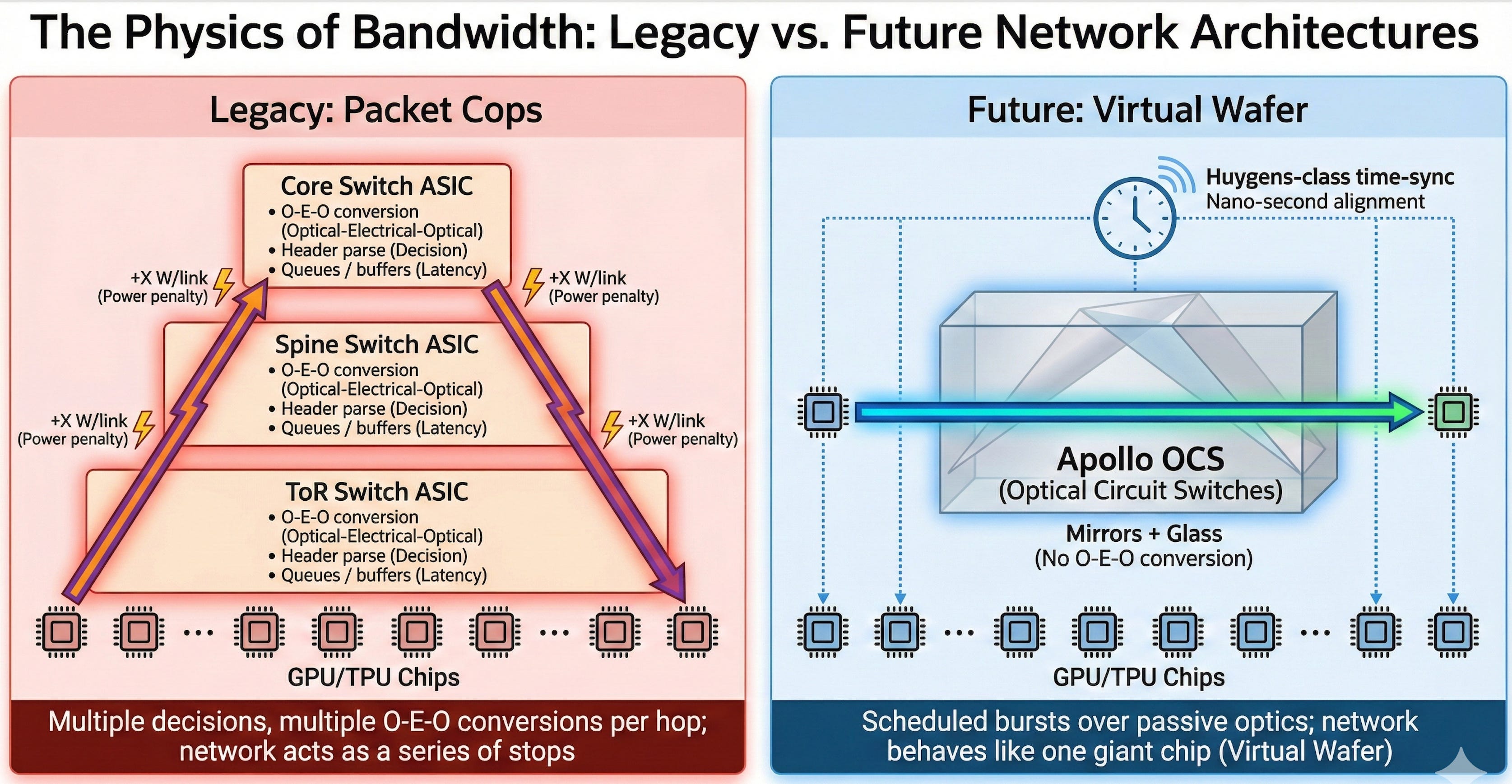
3) The Physics of Bandwidth: From Packet Cops to Virtual Wafers
The constraint in networking isn’t the speed of light; it’s how often you stop light to think about it. Every time a photon becomes an electron and passes through a switch ASIC, you pay in power (O‑E‑O conversion) and latency (indecision). Treat a data center as a bunch of servers, and this is just “networking gear.” Treat it as a Virtual Wafer—one giant computer—and the network is the computer. The “Idiot Index” of the legacy design is how many times you turn light into heat and back into light just to move a tensor from Chip A to Chip B.
Google’s 1,000× roadmap on the network side is really about deleting decision points. Apollo’s optical circuit switches (OCS) already rip out big layers of electrical spine switches; Google’s Huygens‑style time‑sync stack gives you tens‑of‑nanoseconds clock alignment so collectives can be scheduled instead of guessed. The next questions are: what can you delete at the rack and pod level, and how do you make sure the fabric respects the SPAD split—Readers vs Writers, prefill vs decode—instead of fighting it?
Phase 1 – Deconstruct to Physics: The SerDes Tax & The Reactive Trap
Two physical realities dominate the cost of moving bits today:
The SerDes tax. SerDes (serializer/deserializers) and their DSP front‑ends encode wide, slow on‑chip data into multi‑GHz streams on copper. At 400–800 G and beyond, those blocks are chewing up on the order of 30% of the I/O power budget on many modern parts—more and more of the chip’s thermal envelope is spent fighting signal loss and jitter rather than doing model math.
The reactive trap. Traditional switches exist to manage randomness: they read headers, juggle queues, and make per‑packet decisions because internet traffic is chaotic. But AI training traffic is not chaotic. It’s a sequence of all‑reduce collectives the compiler knows about in advance. Even inference becomes structured once you apply continuous batching: user requests get buffered into 5–50 ms “trains” so the hardware sees predictable bursts, not white noise. Using fully reactive packet switches for this is like putting stop signs in the middle of a railway.
Even after Apollo deletes the electrical spine, you’re still paying for:
ToR switches that treat each rack as a mini‑internet.
Short‑reach copper between TPUs/NICs and transceivers, which forces additional SerDes and retimers right where the energy per bit is already worst.
Overlay that with workload physics and the SPAD split:
Scale‑out training (“the symphony”) – deterministic bursts: 10k chips compute for ~300 ms, then scream at each other for ~50 ms, then go quiet.
Scale‑out inference (“the factory”) – messy at the user edge, but internally decomposes into:
Reader flows (prefill) – big, matmul‑heavy, compute‑bound.
Writer flows (decode) – small, KV‑cache‑heavy, memory‑bound and tail‑latency sensitive.
If the network ignores that structure and uses the same Clos/ToR logic everywhere, you’ve effectively thrown away half of what SPAD and batching bought you. The job now is to delete as much of that generic machinery as physics will allow.
Phase 2 – Rebuild to Economics: Color, Air, Analog, and Petabyte Shelves
3.1 The Rainbow Bus (Passive WDM) – Routing by Color, Not Silicon
The Rainbow Bus idea asks: if you already know which node you’re sending to, why decode headers at all? Arrayed Waveguide Grating Routers (AWGRs) are passive photonic devices that route light by wavelength: “red” exits port 1, “blue” exits port 2, etc. Combine them with fast tunable lasers and you get a wavelength‑routed fabric: the TPU doesn’t send a packet “to chip #50,” it just emits on λ₅₀ and the glass prism sends it to the right place. No switch ASIC, no O‑E‑O, essentially zero incremental power to route.
Reality check:
AWGRs are mature enough for telecom and have been prototyped for data center networks. The physics is sound, but crosstalk, temperature sensitivity, and wavelength management make it hard to scale them to thousands of ports without heroic engineering.
Fast, stable tunable lasers exist in research and early products, often using microcombs or integrated photonics, but they’re still expensive and tricky to manufacture at hyperscale.
Where it makes sense soon is not as a planet‑scale “Rainbow spine,” but as a pod‑scale delete:
Use AWGRs inside a pod or rack‑group to replace ToR switches and some SerDes: 32–64 nodes can be interconnected via a passive wavelength fabric. Training and prefill traffic—static, compiler‑known patterns—are a perfect match.
The compiler (XLA/Pathways) assigns wavelengths deterministically: rank 0 sends gradients on λ₀, rank 1 on λ₁, and so on. The fabric becomes a static “color map” rather than a programmable router.
In SPAD terms, the Rainbow Bus is most valuable for Reader and training pods. It lets you treat a pod as a fully connected clique without paying a kilowatt of ToR silicon. For Writers and latency‑sensitive decode, the routing problem is different; static wavelengths are less compelling there. So: keep Rainbow at pod/rack scale, wired into training/prefill, and don’t pretend it can replace Apollo’s OCS core in the campus anytime soon.
3.2 The Breathing Fabric (SerDes Power‑Gating)
Google already knows networks ‘breathe’: long compute phases, short communication bursts. Its Huygens‑class time‑sync stack gives every NIC and TPU a shared notion of ‘now’; Apollo’s mirrors reconfigure in milliseconds before a collective starts. That’s enough to turn the network into a scheduled organ rather than a static utility.
The obvious first principle move is: stop powering lungs that aren’t inhaling.
You can’t hard‑off standard WDM lasers without dealing with wavelength drift and relock time, but you can power‑gate the hungry SerDes and DSP electronics for long stretches.
The scheduler knows when all‑reduces are coming, and in inference land, the batcher knows when big prefill waves will hit. In the gaps, NICs can put high‑speed I/O blocks into deep sleep, only waking in time to reacquire clocks and align CRCs.
Across hundreds of thousands of links, that’s not rounding error; it’s megawatts. And it’s purely a software + firmware change on top of existing optics. This is low‑hanging fruit for Amin’s 4–5‑year window: fully compatible with Apollo and Falcon, and complementary to everything else.
3.3 SPAD‑Aligned Networks: Reader Pods, Writer Pods, and the Cortex
Where the previous drafts were too generic, this is where we tie networking directly to SPAD.
Reader Pods (Prefill). These are Ironwood/Trillium‑heavy clusters optimized for matmuls: lots of compute, enough HBM to hold weights, and very high bandwidth for one‑shot prompt ingestion. Their outbound traffic is mostly compact state (KV/cache summaries) headed to Writers. They benefit from pod‑local Rainbow Bus or similar static fabrics and from Apollo‑style scheduled optics when they ship state across the campus.
Writer Pods (Decode). These look like “HBM with a brain”: lots of memory and KV cache, modest compute. Their network priority is low‑tail‑latency, many‑to‑one links to memory tiers and KV/state stores, not massive bisection bandwidth. Inside a Writer pod, the “network” should look more like a CXL/photonic memory fabric than like Ethernet; the main job is to keep KV cache and agent state electrically close, not to route arbitrary RPCs.
Cortex Tiles (State). For long‑lived agents, you want a small number of SRAM‑heavy “cortex” pods where context and world‑model live essentially permanently. Networking’s job is to keep Reader/Writer compute gravitating toward the cortex that holds a session’s state, instead of reloading context from cold storage on each turn.
Topology‑aware scheduling is the glue: the orchestrator places a user’s session on a specific Writer + Cortex neighborhood and keeps it there, minimizing cross‑campus hops and avoiding “KV ping‑pong” across pods. That’s a simple software policy, but it demands explicitly SPAD‑aware fabric design, not a generic L3 mesh.
3.4 The Air‑Gap (Indoor FSO) – When Fiber Runs Out
Bringing Project Taara indoors is exactly the kind of off‑script move Amin would appreciate: delete cable bundles, beam bits through air. Research prototypes like FireFly and OWCell show that rack‑to‑rack free‑space optics (FSO) in a data center is possible: steerable laser “eyes” on racks hitting ceiling mirrors, reconfigurable in software.
But reality bites:
Line‑of‑sight can be blocked by people, lifts, new racks.
Dust, smoke, and refractive turbulence affect reliability.
Aligning and maintaining thousands of beams in a hot, vibrating hall is non‑trivial.
So the right framing is: FSO is a scalpel, not a backbone.
Use it as a “break glass” overlay where you literally can’t pull more fiber (heritage buildings, constrained conduits, brownfield retrofits).
Use it to temporarily augment bandwidth between hot pods while permanent optical fibers are being added.
For Amin’s 1,000× plan, FSO is a niche tool. It’s clever and occasionally necessary, but the main line should be more glass and smarter fabrics, not turning every row into a room full of Taara turrets.
3.5 The Petabyte Shelf (Optical CXL) – Fixing the Memory Wall for Writers
The Petabyte Shelf is the least speculative idea here and the most aligned with what the ecosystem is already building. Today, HBM is bolted to the accelerator. If one chip runs out of memory, it fails, even if its neighbor has tens of gigabytes free. CXL (Compute Express Link) and related standards exist precisely to turn memory into a pooled resource, and photonic I/O vendors like Ayar Labs and Celestial AI are explicitly targeting optical memory fabrics that detach DRAM from compute.
The architecture looks like this:
A rack (or short row) of memory sleds: DRAM/NVRAM shelves attached via CXL or a custom photonic protocol.
Ironwood/Trillium tiles with optical I/O chiplets that talk load/store semantics to those shelves—“read 4 MB from slot X”—instead of slinging giant KV blobs over IP.
A controller layer that manages allocation, QoS, and basic coherency.
SPAD‑wise, this is the missing organ:
Readers keep most of their weights and temporary activations in local HBM but can spill rare big layers or long contexts to the shelf.
Writers treat the shelf as their primary KV/agent state store, pulling the hot working set into local SRAM/DRAM and leaving the rest in pooled memory.
Cortex tiles effectively live in the shelf: long‑lived agent state is just a pinned region of this pooled RAM.
Feasibility is high:
CXL memory pooling is already shipping in CPU systems; hyperscalers are deploying it for databases and in‑memory analytics.
Celestial AI and Ayar Labs both report hyperscaler engagements to build photonic fabrics for disaggregated memory and accelerator I/O.
For decode and agent workloads, this is the most direct path to a 10×–100× effective memory increase without 10×–100× more HBM stacks and power.
3.6 The Analog Sum – Where to Park It (For Now)
Analog optical computing—doing math with interference, not transistors—is very real in the lab. Groups and startups have shown optical matrix‑vector multiplies, convolutions, even pieces of backprop, and you can absolutely build an optical adder tree that performs a reduce‑sum across a few dozen inputs “for free” in the optical domain.
The problems are precision and scale:
Gradient sums need ~8–16 effective bits of accuracy over wide dynamic ranges; analog optics adds noise, drift, and calibration overhead.
Integrating large optical mesh networks into real TPUs and routing gradients through them without massive engineering risk is a long project, not a 2‑year rollout.
The sensible compromise is:
Treat analog sum as a near‑chip or rack‑level accelerator: use optics to pre‑aggregate gradients from a handful of neighbors, then feed the result into a digital all‑reduce tree. That shrinks data volume and I/O energy without betting training convergence on a fully analog fabric.
Keep it in the Phase 3/R&D bucket for Amin’s plan. It’s aligned with physics, and DeepMind‑style algorithmic robustness might make it viable sooner than people expect, but it’s not something you count on for 2029 capacity.
The Profound Bit: What Google Should Actually Do
If you strip away the sci‑fi and keep only what the physics and timelines support, the networking playbook that maximizes value for Google looks like this:
In training:
Double down on Apollo + Huygens as the “optical scheduler” for pods and campuses.
Push co‑packaged optics and short‑reach photonics to delete as much SerDes tax as possible.
Experiment with Rainbow‑style AWGR fabrics inside pods to delete ToRs and let the compiler assign wavelengths.
Add breathing‑fabric power‑gating to SerDes and DSPs to reclaim idle megawatts.
In inference:
Make SPAD real at the network level: physically distinct Reader, Writer, and Cortex pods, with topology‑aware placement of agent sessions.
Build Petabyte Shelves—CXL/photonic memory fabrics—that take KV and context off local HBM and turn them into pooled assets.
Use Apollo + batching for long‑haul state moves; use memory fabrics, not IP meshes, for most Writer and Cortex traffic.
In research:
Treat Rainbow Bus at campus scale, Air‑Gap fabrics, and full analog all‑reduce as high‑upside experiments, not prerequisites. Fund them through DeepMind and the hardware research org as 2030s accelerants, not 2020s dependencies.
That way, networking stops being a static cost and becomes another place where first‑principles design can buy you orders of magnitude. Not by buying more 800 G ports—but by deleting the parts (ToRs, unnecessary SerDes, generic meshes) that no longer make sense once you accept that an AI data center is not a collection of servers. It’s a Virtual Wafer, and the job of the network is to make that lie as close to true as physics allows.
What this means for investors: follow the glass, not the cops
If you take the Virtual Wafer idea seriously, the center of gravity in networking shifts away from “smart packet cops” and toward photons, packaging, and memory fabrics.
The legacy trade was: buy the switch ASIC vendors and assume complexity scales with bandwidth. But in a spine built around Apollo‑style OCS and Huygens scheduling, the whole point is to delete routing intelligence from the middle of the fabric. The value is migrating up into the compiler/runtime (Pathways, XLA, vLLM‑style batching) and down into the optics and materials that make a glass core viable for 10–15 years. The risk, from an investor’s lens, is being long on companies whose only differentiation is “smarter packet inspection in a Clos spine” as hyperscalers quietly replace those spines with passive mirrors and wavelength fabrics.
The upside is in the supply chain that makes Virtual Wafers and Petabyte Shelves real. That means optical engines and CPO, not just pluggables; photonics assemblers and test houses (the “TSMC of the network”); electro‑optic bridge silicon for CXL and memory pooling; and the materials and fiber vendors whose volume explodes if every large campus needs tens of thousands of strands between buildings instead of a few hundred. Your mental rotation is: from “ports per switch” to watts per bit, from “L3 features” to how early can we turn electrons into light and never turn them back until we hit HBM or DRAM. The companies that win that game, even if they’re small today, are the ones that will quietly sit under every Reader pod, every Petabyte Shelf, every campus‑scale Virtual Wafer.
What this means for data center operators: design for fiber gravity and SPAD zones
For operators, the big shift is that topology and conduit become as critical as megawatts and floor loading. If your mental model is still “roomful of identical halls with standard 4″ duct banks between them,” you’re not building for Virtual Wafers. A 100k‑chip training cluster spread over two or three buildings wants absurd fiber density and very clean, low‑loss paths: straight‑shot duct banks, room for multiple high‑count cables, and the physical plant to support OCS nodes and optical patching at campus scale. You’re not just sizing transformers; you’re engineering fiber highways.
SPAD also implies you stop treating every white space the same. Reader pods (training + prefill) want very high rack densities, liquid cooling, short hop latency into the optical core and maybe Rainbow‑style pod fabrics. Writer pods and Petabyte Shelves want memory density, CXL backplanes, and clean short‑reach optics more than insane kW/rack. Cortex/state pods want ultra‑reliable power, low‑latency fabrics, and tight coupling to storage. The operator who can walk into a Google/Anthropic/Cohere RFP and say, “Here’s our Training Zone spec, here’s our Inference/Writer Zone spec, here’s our Memory/Shelf pod spec, and here’s the duct bank between them” is playing a different game than the one still selling “up to 10 kW per rack, chilled water available”.
This is also where campus layout becomes a moat. If you have brownfield campuses with existing high‑capacity duct, rights‑of‑way for new fiber, good line‑of‑sight between buildings (for the odd FSO overlay), and the physical volume to host OCS/patch rooms, you can credibly market yourself as Virtual‑Wafer‑ready. If you don’t, the cheapest thing you can do today is overbuild conduit and risers everywhere you still can; the most expensive thing you can do is assume “a couple of 864‑count bundles between halls” will be enough when Reader/Writer clustering and Petabyte Shelves really show up.
What this means for colos & developers: sell fabric‑ready shells, not just space & power
For colocation providers and developers, the networking deep dive basically says: “space and power” is table stakes; the product now is fabric readiness. Your best tenants over the next decade will be AI shops that aren’t quite big enough to build their own Jupiter+Apollo clone, but want something that rhymes with Google’s architecture.
That means three things. First, your MMR and campus interconnect story has to level up. It’s not just “here are the IXPs and waves we can sell you”; it’s “here is a pre‑engineered optical mesh across our buildings, with dark fiber or wavelength services you can treat as your own Virtual Wafer core”. If you can offer OCS‑friendly topologies or even managed optical fabrics between suites—“here’s a 4‑hall mesh with guaranteed latency and loss characteristics, ready for your Reader/Writer split”—you’ll win training and stateful inference workloads that a vanilla colo never sees.
Second, you can start to productize SPAD in real estate terms. Instead of generic 2 MW halls, you market:
“Training Suites”: liquid‑ready, high floor loading, dense power distribution, great cross‑connect into the campus glass core.
“Inference / Edge Suites”: more modest power, but rich metro connectivity and short paths to MMRs and end‑user networks.
“Memory / Shelf Suites”: optimized for Petabyte Shelves and CXL fabrics, with lots of rack positions, moderate power, and very clean, short‑reach optical paths to adjacent compute suites.
Third, you can differentiate by being the neutral aggregator of weird infra that makes these fabrics possible. Most AI tenants don’t want to negotiate for extra duct banks, exotic fiber types, shared Petabyte shelves, or FSO links across roofs with landlords and cities; they want someone who shows up with a “cluster‑ready envelope.” This is where working with FPX‑type partners helps: you show up not just with powered land, but with pre‑sourced optical plant, duct, and even shared memory/caching tiers they can plug into. In a world where hyperscalers are turning their own DCs into Virtual Wafers, the edge for colos is to offer the same pattern—glass core, SPAD‑aware zoning, pooled memory—without the tenant having to reinvent Jupiter in a leased hall.
This is the fourth and final “Physics” deep dive. We have covered Chips, Power, and Networking. Now we tackle Memory.
The “First Principles” hook here is: Memory is the only thing that matters.
Compute is cheap ($10^{-12}$ Joules). Moving data from memory to compute costs $100\times$ more energy. The “Memory Wall” is not a metaphor; it is a thermodynamic tax.
4) The Physics of Memory: HBM Is the New Oil (and We’re Wasting It)
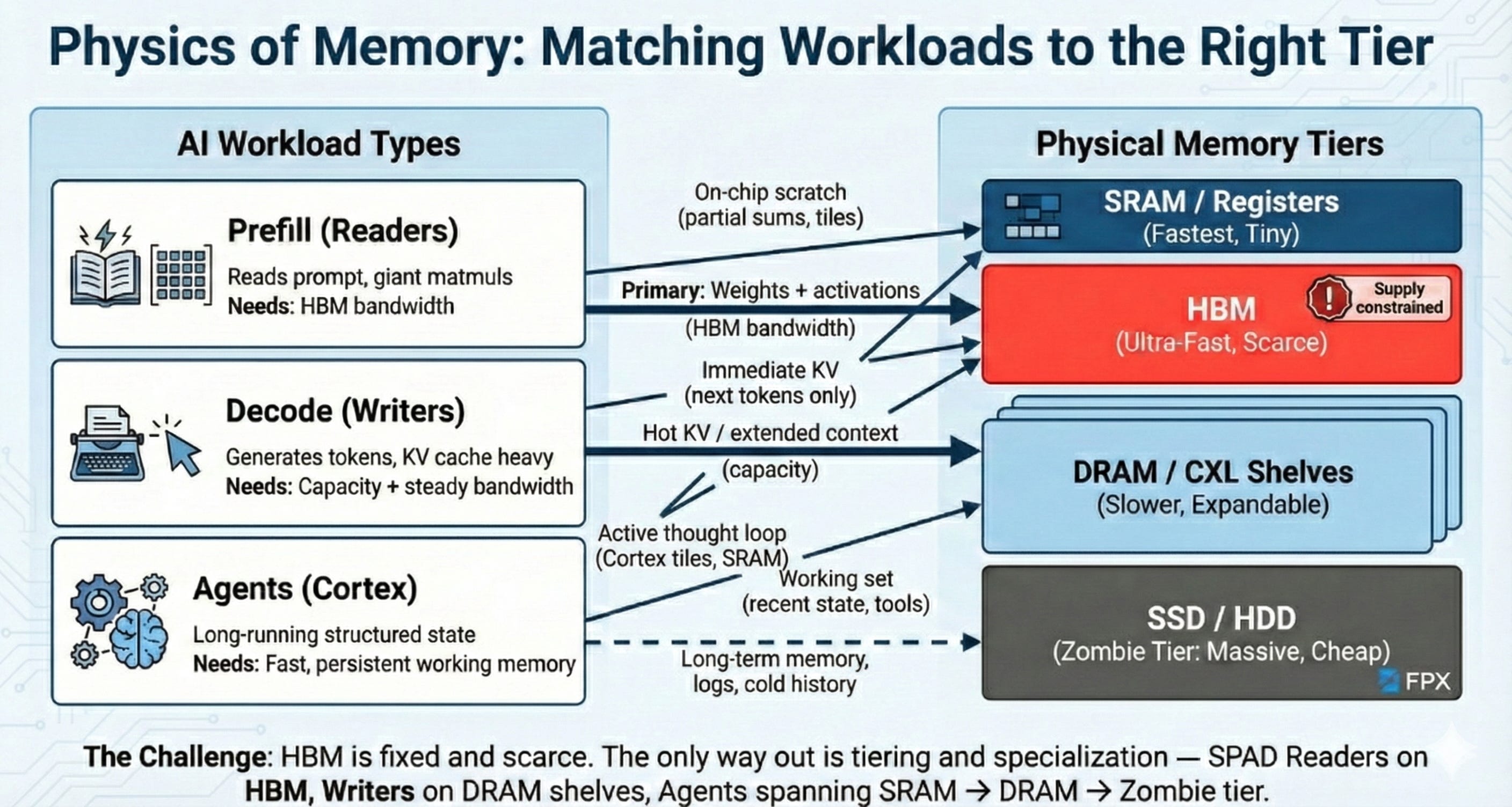
We went deep on this in our earlier piece, Beyond Power: The AI Memory Crisis – arguing that the real constraint on hyperscale AI isn’t how many GPUs you can buy, but how many useful bytes you can keep close to them and at what cost. That piece mapped the DRAM/HBM supply chain, the CoWoS bottleneck, and why memory has become the hidden governor of AI scale. Here, we take that a step further and apply a first‑principles lens specifically to Google’s world: HBM scarcity, SPAD (prefill vs decode), agents, and how a company at Google’s scale can architect around a memory system it does not fully control.
If you strip Google’s AI stack down to physics, one thing jumps out: compute is no longer the limit — memory is. A TPU or GPU can do a low‑precision MAC for a fraction of a picojoule; the expensive part is hauling the operands in and out of memory. Every rung you climb down the hierarchy, from SRAM to HBM to DRAM to SSD to HDD, adds orders of magnitude in energy and latency. In a large LLM, most of the joules are spent moving bits, not thinking with them.
Now add the supply chain: the only memory fast enough to keep up with frontier chips is HBM (high‑bandwidth memory), and that market is tiny and stressed. SK hynix has become the HBM kingpin, Samsung has most of the remaining share, and Micron, after largely sitting out the early HBM3 cycle and focusing on HBM3E — is only now ramping into contention. Packaging (TSVs, 3D stacking, 2.5D interposers) is the real choke point, and all three vendors have broadcast the same message: HBM capacity is effectively sold out into the mid‑2020s. One of the three skipping a full generation (HBM3) is precisely why the shortage feels so acute.
HBM is now the most expensive real estate in the data center on a per‑bit basis, yet the way we use it looks like a landlord who rents skyscrapers to people who only occupy half a floor. We solder 80–192 GB of HBM to every accelerator and then strand a huge fraction because the workload doesn’t perfectly fill the silo. That’s the memory Idiot Index: the scarcest, hardest‑to‑scale resource is also the least efficiently used.
If Google applies a genuine first‑principles framework here — question every assumption instead of importing GPU culture — it has to behave as if HBM supply never really catches up. That means:
Treat HBM as a cache, not a comfort blanket.
Design memory around the actual structure of LLM workloads: prefill vs decode vs long‑running agents.
Push everything that doesn’t absolutely need HBM into DRAM, SSD, HDD, and older silicon that FPX can scavenge.
Phase 1 – Deconstruct to Physics: Prefill, Decode, Agents vs HBM
Start with what the model actually does.
Prefill (Readers)
Reads the full prompt and context.
Giant matmuls and dense attention; access patterns are wide and relatively predictable.
Extremely sensitive to HBM bandwidth and locality.
This is where HBM earns its keep.
Decode (Writers)
Generates tokens one (or a few) at a time.
Dominated by KV cache and attention over the past tokens.
Mostly memory‑bound; compute units wait on KV and embeddings.
Needs capacity and steady bandwidth more than bleeding‑edge FLOPs.
Agents (Cortex)
Long‑running workflows: coding agents, planners, research assistants.
Need consistent, structured state over minutes or hours.
Working set is relatively small but hit constantly; the rest is long‑term memory.
Now overlay the physical tiers:
SRAM / registers — nanoseconds, tiny energy, minuscule capacity, very expensive area.
HBM — ultra‑fast, low latency, horrifically expensive and supply‑constrained.
DRAM / CXL shelves — larger, slower, still decent energy/bit; expandable.
SSD / HDD — massive, slow, cheap; lots of used capacity in the world.
And the key constraint: HBM output can’t be scaled at will. Micron sitting out much of HBM3 and only going big on HBM3E means one entire slice of potential supply simply wasn’t there when AI demand took off. SK hynix and Samsung are already maxing their TSV/stacking capacity. There is no “we’ll just get another 3× HBM by 2027” button.
So the first‑principles conclusion is:
You cannot scale prefill, decode, and agents by just slapping more HBM on each chip.
You have to change how each stage uses HBM and push everything else into tiers FPX can actually source at scale.
Phase 2 – Rebuild to Economics: SPAD‑Aligned Memory in a Scarce‑HBM World
Now we rebuild the memory hierarchy with two constraints in mind:
HBM is a fixed, cartel‑constrained resource.
Prefill, decode, and agents have totally different physics.
4.1 Prefill (Readers): HBM‑only, at 4 bits whenever possible
Prefill is the only stage that truly deserves HBM by default. That means:
HBM holds only hot weights and minimal activations.
No KV caches. No agent history. No long prompts.
If a byte isn’t repeatedly touched in microseconds, it gets evicted to DRAM/SSD.
Virtual HBM with FP4/INT4.
Prefill is mostly linear algebra in well‑behaved layers. This is the easiest place to go aggressively low‑precision.
Make FP4 / INT4 the default for Reader weights and activations; reserve FP8/BF16 only for the genuinely sensitive layers.
For the tensors that can move from 16‑bit to 4‑bit, you get up to a 4× shrink in footprint. In practice, you might see something more like 2–3× effective capacity once you blend in FP8/BF16 layers, metadata, and uncompressed tensors — but even that is the difference between ‘HBM as a hard wall’ and ‘HBM as a tight but manageable budget.
Pod‑level HBM pooling.
Stop thinking “1 chip = 1 silo.” Treat the prefill pod as a shared HBM pool.
The compiler/runtime should pack layers and shards across devices so you never have one 80 GB HBM stack 30% full and another spilling.
The subtle but important bit: this locks in a design target for DeepMind and Gemini. “Train so that the prefill path runs at 4 bits” is not just a modeling trick; it’s a hard requirement to keep the HBM budget survivable.
Our contention is that better‑curated, Gemini‑cleaned corpora are what make 4‑bit training practical at scale; the data pipeline becomes part of the hardware strategy.
FPX doesn’t touch HBM directly, but by helping Google push everything else into cheaper tiers, it gives Amin room to be ruthless here: HBM is only for this narrow prefill hot path.
4.2 Decode (Writers): stop using HBM as KV landfill
Decode is where current systems quietly torch HBM on the wrong work: KV cache, bloated contexts, scratch state.
For Writers:
Default assumption: KV and long context do not belong in HBM.
Keep the immediate KV needed for the next few tokens on HBM.
Everything else — older KV blocks, extended context windows, multi‑agent scratchpads — gets pushed into DRAM via CXL Petabyte Shelves.
Use CXL shelves as “decode lungs”, not fake HBM.
A decode node might have 64–96 GB HBM for weights and hottest KV, and borrow 512 GB–1 TB of pooled DRAM from a CXL shelf.
CXL DRAM is ~100–200 ns slower than local DRAM, but for older KV/less frequently accessed context it’s still orders of magnitude better than going to SSD.
Compress and summarize KV aggressively.
Blockwise quantization, sparse KV, dynamic truncation, and summarization can slash the footprint.
The less KV you store per token, the less HBM/DRAM you need per 1 M tokens served.
Here FPX can directly help:
FPX can work with distressed operators, OEM buyback programs, and decommissioned fleets to acquire memory‑heavy servers (lots of DIMMs, older CPUs).
FPX tests and bins the DRAM, and bundles them as CXL shelf bricks—pre‑packaged DRAM pools Google can drop behind decode pods.
That’s a clean division of labor: Google solves the software and scheduling; FPX solves, “Where do we get a few petabytes of cheap DRAM in the next 18 months?”
4.3 Agents (Cortex): SRAM for thought, junk for long‑term memory
Agents are where “reload everything from disk every turn” becomes untenable.
First‑principles fix:
Introduce Cortex tiles — SRAM‑heavy chiplets per pod.
Reserve a small number of tiles with tens/hundreds of MB of SRAM and some HBM for agent working sets.
High‑value agents get pinned to a Cortex tile for the duration of their job; their active plan, stack, and short‑term memory never leaves silicon.
Tier agent memory by actual access frequency:
SRAM: active thought loop, recent messages, immediate code.
HBM/DRAM: last N steps of history, hot tools and docs.
SSD/HDD (Zombie Tier): logs, old context, rarely used references.
Again, this forces modeling and infra choices: agents must be designed to keep their “mind” small: compressed latent representations and summaries that fit in limited SRAM, not 10 GB JSON blobs.
FPX’s part is to make the bottom of this pyramid feel infinite and cheap:
Zombie SSD/HDD clusters right next to agent pods, built from recertified drives and retired JBODs.
Cheap capacity for all the stuff agents might need twice a month but which should never be on HBM or even DRAM.
4.4 The Zombie Tier: where FPX lives
The Zombie Tier is where FPX can provide immediate, non‑theoretical value:
Checkpoint Pods.
Training checkpoints are huge sequential writes with rare reads.
FPX can aggregate retired enterprise HDDs and SSDs (via direct buys, OEM recert programs, and structured buybacks), wipe and test them, then sell them back as “Checkpoint Pods” with clear SLAs: cheap, sequential, redundant.
Cold Context Pods.
Old agent histories, low‑frequency RAG corpora, archived models.
Same underlying hardware, different durability/availability profile.
Instead of Google burning fresh NVMe at $X/TB on workloads that don’t need it, FPX feeds in Zombie capacity at a fraction of the capex and keeps that spend focused on HBM/DRAM where the whole world is truly constrained.
FPX Zombie Tiers: Cheap bytes that free scarce HBM.
Checkpoints want sequential I/O and redundancy, not fresh NVMe. Agent histories want cheap depth, not sub‑100 ns latency. FPX aggregates recertified SSD/HDD into Checkpoint Pods and Cold Context Pods with clear SLAs, so HBM and DRAM stay reserved for prefill/compute and hot KV. Result: more usable tokens per joule and fewer wasted HBM silos.
4.5 “Zombie GPUs”: only for long‑tail inference, not as cache bricks
Your pushback is exactly right: using older GPUs as glorified HBM cache bricks is thermodynamically dumb. An A100 idling just to keep its HBM online still burns serious power; a DRAM DIMM or CXL shelf is far more efficient if all you want is capacity.
So the first‑principles rule should be:
Never run a 300 W GPU just to emulate a 5 W DRAM stick.
Where “Zombie GPUs” do make sense is in long‑tail inference, where you still need both compute and memory bandwidth, but not the latest perf/W:
Serving small or mid‑sized expert models, older Gemini generations, or internal tools where latency isn’t hypersensitive.
Batchy, background workloads like email summarization, internal analytics, or low‑priority agents.
These are jobs where you’d otherwise be tempted to “waste” H100s or newest TPUs. Instead, FPX can:
Scoop up A100/H100/older TPU fleets from neoclouds and failed AI startups.
Stand them up as Long‑Tail Inference Clusters in power‑cheap sites.
Let Google and others offload non‑critical workloads there so the newest HBM is saved for frontier pretraining and high‑value inference.
Framed that way, Zombie GPUs are not “memory nodes”; they’re a way to avoid burning fresh HBM on tasks that don’t need it. Anything that really is “just cache” should be pushed down into DRAM/SSD via shelves and Zombie Pods.
FPX Long‑Tail Clusters. We stand up retired accelerators in power‑cheap sites for throughput LLMs, batchy internal jobs, and non‑critical inference—so frontier TPUs stay on frontier work.The FPX Layer: Turning Scrap Silicon into Usable Memory
Across all of this, FPX’s role is pretty clear:
Used SSD/HDD sourcing and aggregation
Work directly with hyperscalers, colo providers, and OEM recert programs to set up buyback channels.
Turn that into standardized Checkpoint/Context Pod SKUs.
Used DRAM and servers for CXL shelves
Acquire memory‑dense servers from distressed operators and refresh cycles.
Test, bin, and ship them as “Shelf Bricks” tailored for Google‑style decode pods.
Zombie GPU clusters for long‑tail inference
Aggregate old accelerators and sell them explicitly as “Good enough inference for X $/token” capacity, not as generic GPU hours.
Partner with OEMs up the chain
Cooperate with drive and memory vendors on structured buyback/refurbish programs so they get ongoing margin and FPX gets predictable supply.
If Google wants a first‑principles answer to the memory bottleneck, it looks something like this:
Assume HBM will stay scarce and expensive.
Design SPAD architectures — Reader, Writer, Cortex — to need as little of it as possible.
Push everything else down into DRAM and junkyard silicon.
Let FPX handle the ugly work of turning the world’s retired drives, DIMMs, and GPUs into clean, productized Zombie tiers.
That’s how you stop treating HBM like a commodity you’ll always be able to buy more of, and start treating it like what it really is: the limiting reagent in the 1,000× AI experiment.
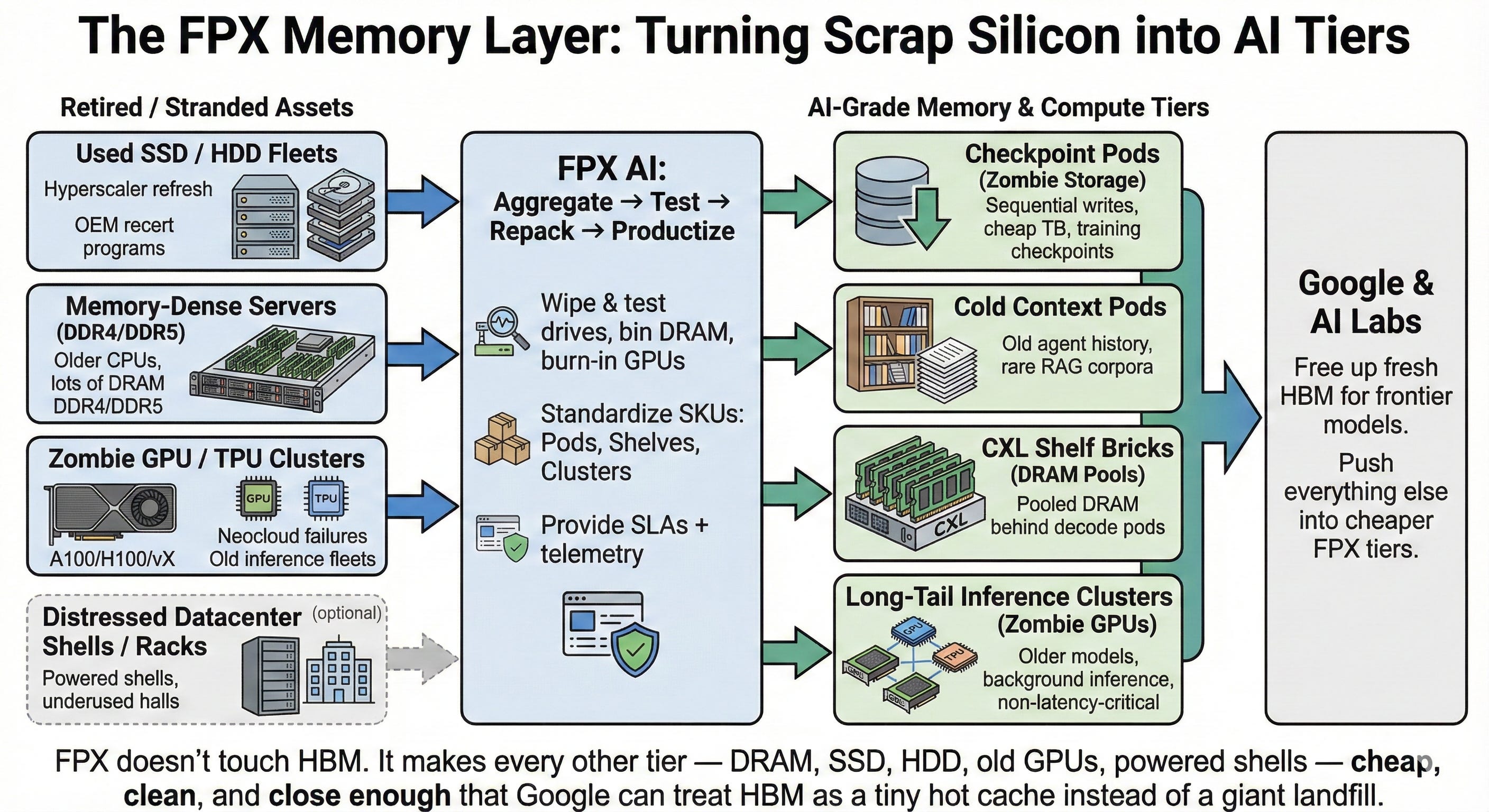
What this means for investors
For investors, the memory story says: HBM is the new oil, but the real upside is in everything that makes us need less of it. The obvious plays (SK hynix, Samsung, Micron, HBM packaging/CoWoS houses) are already priced as if they are the only game in town—and they are the bottleneck—but the asymmetric opportunities are around them: CXL and memory‑pooling silicon (Astera‑style), photonic/copper interconnects that make Petabyte Shelves viable, and the testing/recertification ecosystem that can turn “used” SSDs/DRAM into Zombie Tiers with credible SLAs. The winners aren’t just the ones selling fresh HBM; they’re the ones selling more useful bytes per HBM bit—through FP4, pooling, compression, and “good enough” capacity from refurbished hardware. FPX AI sits squarely in that second category: if it becomes the default aggregator and seller of “AI‑grade used memory and storage,” it captures a structural margin from everyone who is still buying brand‑new flash and DRAM for checkpointing and cold data.
What this means for data center operators
For data center operators, the takeaway is that memory topology becomes as important as power and cooling. A campus that wants to host serious AI can’t just offer “GPU cages”; it needs SPAD‑aware memory zones: high‑bandwidth, low‑latency adjacency between Reader pods and their HBM‑first racks; separate decode/Writer rows with space and power for CXL Petabyte Shelves; and colder storage rooms (lower power density, lots of rack positions) for Zombie Tiers built from HDD/SSD. That means planning for more east–west connectivity between compute and memory racks, designing “shelf rows” and “checkpoint rows” explicitly, and being willing to let a partner like FPX drop in pre‑assembled shelf bricks and checkpoint pods sourced from the secondary market. The operator that can say, “We have dedicated space, power, and fiber for your pooled DRAM and cheap checkpoint capacity, not just for your TPUs,” will win the tenants who understand that HBM is scarce and everything else has to move closer and get cheaper.
What this means for powered‑land and infrastructure owners
For powered‑land owners—people sitting on substations, stranded power, old industrial sites—the memory lens opens up a new product: “memory campuses” rather than just “compute campuses.” Petabyte Shelves and Zombie storage don’t need the same pristine, ultra‑dense power and cooling as frontier HBM clusters; they need lots of reasonably priced MWs, floor space, and enough connectivity to sit one or two network hops from the main AI site. That makes brownfield sites with decent grid hooks and cheap land—old industrial parks, retired factories, secondary metros—ideal for DRAM shelves and checkpoint pods. FPX can sit in the middle: taking those powered shells, filling them with refurbished DRAM/SSD/HDD capacity and CXL‑ready nodes, and then presenting them to hyperscalers and neoclouds as “off‑site memory extensions” that free up premium metro real estate (and HBM budget) for Readers, Writers, and Cortex tiles. In other words: powered land that can’t justify a 100 kW/rack GPU build can still be extremely valuable—if it brands itself as the cheap, deep memory layer under someone else’s scarce HBM.
5) Model Evolution: Turning Physics into Intelligence
Everything we’ve laid out so far — TPUs, power, networking, memory — buys Google raw 1,000× compute. Whether that turns into 1,000× more intelligence depends entirely on what sits on top of it: the models.
The last 18 months have quietly changed the rules here.
DeepSeek showed that standard Transformers are physically wasteful: their MoE + MLA stack cuts KV memory and active compute massively versus dense baselines while matching or beating quality.
DeepSeek‑R1 and OpenAI o1 showed that thinking longer at inference can matter more than making the base model bigger: chain‑of‑thought and test‑time compute become primary scaling axes.
Google’s Titans work showed how to break the context window trap with learned neural memory — separating short‑term attention from long‑term, updateable memory at test time.
All three are really saying the same thing in different ways:
The old “just add parameters and pre‑training FLOPs” era is over.
The new frontier is physics‑aware, inference‑time‑aware, memory‑aware models.
So let’s run the same two‑step playbook we used on hardware.
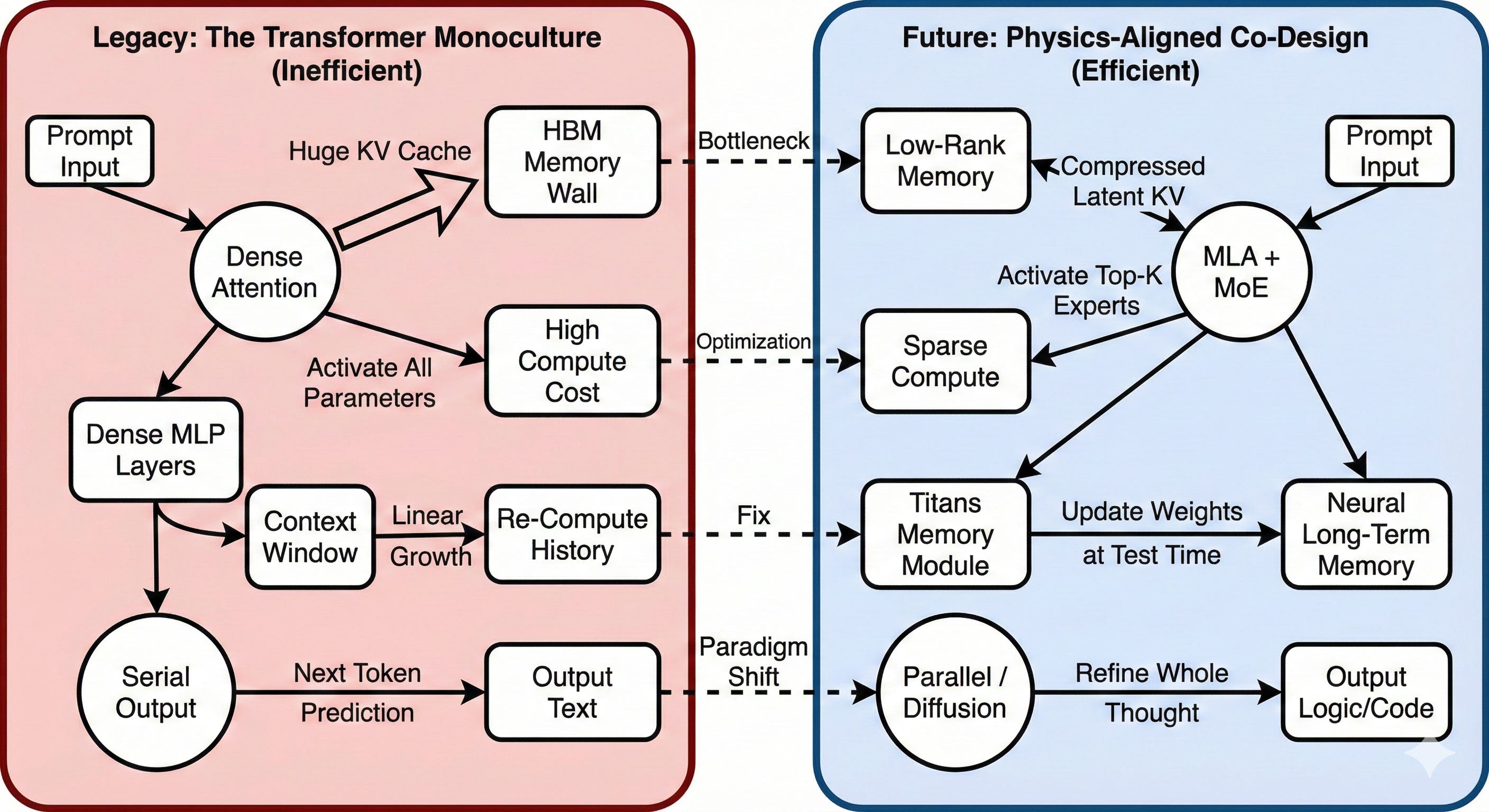
Phase 1 – Deconstruct to Physics: Where Models Fight the Machine
If you strip a standard LLM + agent stack down to what it physically does, the misalignments with Google’s hardware are obvious:
Uniform depth & dense activation
Every token goes through the full depth of the network, and almost every parameter fires. Easy tokens (“the”, boilerplate) pay the same compute and memory cost as hard reasoning steps. That’s maximum FLOPs, maximum HBM churn, maximum SerDes activity — the opposite of what we want on a power‑ and bandwidth‑constrained TPU fleet.KV cache and context as the only memory
Classic Transformers stuff everything into the context window: recent conversation, long‑term history, scratchpad, task hints. KV cache grows linearly with sequence length and heads; by the time you’re playing with 128k+ tokens, you’re essentially using HBM as a giant circular buffer. That’s exactly the resource we’ve already established is the scarcest in the stack.Answer time tied to token count
Autoregressive generation is intrinsically serial: to produce T tokens, you pay at least T forward passes. Great for flexibility, terrible for long reasoning chains or huge code edits, and a bad match for Apollo’s scheduled fabric.No notion of “thinking time” as a separate budget
Traditional scaling laws (Chinchilla etc.) focused almost entirely on training compute. R1 and o1 changed that: they show smooth gains from adding inference‑time compute — longer chains of thought — even at fixed model size. But most of today’s infrastructure and models treat inference compute as a fixed cost rather than a policy decision.Agents as thin chat wrappers
Most “agents” today are just loops around an LLM: send full context in, get text out, repeat. All the state lives in tokens and external tools. There’s no compact world model, no dedicated controller, no learned notion of state — which means massive repeated parsing and KV rebuilds.
Contrast that with what DeepSeek and Titans are actually doing:
DeepSeek‑V2/V3: MoE + MLA + mixture‑of‑depth → far fewer active experts per token, compressed K/V so KV cache is tiny, and conditional depth so not every token pays for every layer.
DeepSeek‑R1 / OpenAI o1: explicit test‑time compute scaling; more internal reasoning steps improves performance without touching the base parameter count.
Titans: short‑term attention + neural long‑term memory + persistent memory → context window becomes a front cache, not the whole story.
All three are directly attacking the same physical constraints we’ve been talking about:
HBM and CXL shelves are scarce → compress KV, use sparsity, separate long‑term memory.
Network bandwidth is constrained and scheduled → avoid dense all‑to‑all every token.
Power ceilings are real → don’t fire all experts and all layers on every step.
Memory hierarchy is layered → stop using context windows as the only “memory.”
That’s Phase 1. Now the fun part is Phase 2: how Google can rebuild models to fit the stack it actually has.
Phase 2 – Rebuild to Economics: Optimization Breakthroughs That Align with the Stack
Here are the key moves that matter and age well — the ones that should guide DeepMind’s roadmap if it wants to be directionally correct for the next decade.
1. Make DeepSeek‑style sparsity and MLA the default
Core idea: pay only for the hard parts of the sequence, and move less KV.
Mixture‑of‑Experts (MoE): activate only a handful of experts per token, and learn routing that respects TPU pod boundaries and Virtual Wafer locality. Experts become “organs” pinned to specific slices of the fabric, not amorphous weights scattered everywhere.
Mixture‑of‑Depth: easy tokens exit early; only difficult regions see full depth. That shrinks average FLOPs/token and cuts HBM traffic.
MLA or MLA‑like attention: compress keys/values into a low‑rank latent space so KV cache shrinks dramatically and attention becomes more compute‑bound than bandwidth‑bound.
This is exactly what DeepSeek has already proven under sanctions; Google should treat it as table stakes, not a curiosity. New Gemini/Titans families should have to justify any departure from “sparse + low‑rank KV” the way a chip designer has to justify adding a big new block on die.
2. Treat Titans Memory as the answer to context, not bigger windows
Core idea: context windows are L1 cache, not memory.
Titans already sketches the right structure:
Short‑term attention for immediate local context.
Neural long‑term memory that learns what to store/retrieve across turns and tasks.
Persistent memory encoding more stable knowledge.
Map that onto the hardware we’ve designed:
Short‑term attention ↔ HBM + on‑chip SRAM (Readers/Writers/Cortex).
Long‑term memory ↔ DRAM CXL shelves that FPX helps Google deploy around decode/agent pods.
Persistent memory ↔ SSD/HDD tiers (including Zombie storage) plus external knowledge stores.
Design principle:
New models must be built assuming
“long‑term memory lives in Titans, not in the context window.”
That means training models to write compact latent summaries into Titans Memory and learn to retrieve them — rather than stuffing everything into a sliding 1M‑token window and hoping more HBM shows up from SK hynix.
3. Embrace thinking‑time arbitrage with Cortex tiles
Core idea: System 1 vs System 2 should be a hardware concept, not just a metaphor.
R1 and o1 show that for hard tasks, it’s better to keep the model size fixed and spend more compute at inference on chain‑of‑thought reasoning.
That matches the Cortex tile concept perfectly:
We dedicate small, SRAM‑heavy, stateful TPUs as “thinking cores” where the model can unroll long chains of thought without thrashing HBM or the network.
System 1 traffic (most queries) never hits these tiles: it goes through small, cheap models on Zombie GPUs or low‑power TPUs with tight latency budgets.
System 2 traffic (hard, high‑value queries) is explicitly routed to Cortex tiles, with a configurable thinking‑time budget: “you can use up to N seconds and M joules to think before answering.”
In this world, inference‑time compute becomes a dial the orchestrator can turn, backed by physical resources that make long reasoning efficient rather than catastrophic for HBM and power. That’s exactly what o1/R1 discovered in software; Google has the chance to give it a proper home in hardware.
4. Add fixed‑depth logic modules: diffusion‑style refinement where it helps
Core idea: turn some long outputs into O(1)‑depth problems.
Autoregressive LLMs are inherently O(T) in depth for T tokens. For certain problems — structured plans, proofs, code edits, config diffs — we can do better by:
Letting a base model propose a full candidate solution.
Running a diffusion/flow‑style module that refines that candidate in a small, fixed number of steps, independent of length.
Verifying or scoring the result with another pass if needed.
This is a good fit for Reader TPUs and Apollo: big, regular matmuls over long sequences in a fixed, schedulable number of steps. It doesn’t replace LLMs; it gives Google a way to offload certain “long but structured” tasks from the serial, attention‑heavy path onto a fixed‑depth refinement engine.
The implementation details will change, but the principle will age well:
Wherever you can turn “token by token” into “refine a full candidate in K steps,”
do it. It aligns with scheduled optics, power‑gating, and high FLOP/s TPUs.
5. Use world models for agents, not chats in a loop
Core idea: agents should simulate next state, not re‑parse their entire life every turn.
Right now, many “agents” are just LLMs in a tool loop: stuff history into context, get a response, repeat. World models give you a cleaner, more physical alternative:
Maintain a compact latent world state for the agent: beliefs, goals, working memory.
At each step, predict the next state given an action and new observations, rather than recomputing everything from raw text.
Use LLMs as tools — to interpret inputs, generate text, or solve subproblems — not as the main state machine.
In our stack:
The world model and state live on Cortex tiles + Titans Memory.
The LLM (Gemini/Titans) is a callable expert, not the agent’s core.
Petabyte Shelves and Zombie storage hold long‑term logs, documents, and knowledge; the world model keeps a compressed working set in fast memory.
That gives Google a path to long‑running, low‑power agents that measure progress in “episodes per joule,” not just “tokens per dollar” — an increasingly important metric as compute and power budgets tighten.
6. Co‑Design or Lose: Why This Matters Uniquely for Google
DeepSeek’s constraints were geopolitical: no top‑end GPUs, hard FLOP ceilings. Their reaction — MLA, MoE, training and inference‑time efficiency — is what you get when physics and policy are hard walls.
Google’s constraints are different but just as real:
HBM comes from a duopoly and CoWoS capacity, not from wishes.
Power and cooling are gated by nuclear/geothermal projects, brownfield deals, and FPX‑style scavenging of generators and substations.
Networks are bounded by what Apollo/Firefly/Huygens and photonics can realistically deliver.
Memory beyond HBM depends on DRAM shelves, used SSD/HDD pools, and clever Titans‑style architectures.
The advantage — and the obligation — is that Google controls the whole stack: TPUs, Axion, Apollo, Jupiter, Kairos/Fervo power, Titans Memory, Gemini/Titans models, agents, and (through partners like FPX) even the used hardware and powered land beneath it.
If it treats models as “just another customer of compute,” it will keep getting out‑maneuvered by labs that have to be more efficient. If it treats model evolution as a co‑design problem with chips, power, network, and memory, it can still be the place where physics bends in its favor.
The optimization breakthroughs are clear:
Phase 1 (Deconstruct): admit that vanilla Transformers and naive agents are fighting the hardware — wasting HBM, abusing context windows, and ignoring inference‑time compute as a controllable axis.
Phase 2 (Rebuild): make DeepSeek‑style sparsity/MLA, Titans‑style memory, thinking‑time arbitrage on Cortex tiles, fixed‑depth refinement modules, and world‑model‑based agents the default design assumptions for the next generation of Gemini and beyond.
If Google gets that right, Amin’s “double serving capacity every ~6 months” target stops being a pure infrastructure race and becomes what it should be: a joint optimization of physics and algorithms. The 1,000× story then isn’t “1,000× more FLOPs”; it’s “1,000× more useful reasoning per joule, per byte of HBM, per meter of fiber” — and that’s the only version that will actually scale.
What this means for investors
The big shift is that “buy GPUs” is no longer the whole trade. If DeepSeek, Qwen, o1, Titans, etc. are directionally right, value migrates from raw flops to everything that lets you use flops selectively:
Routing and orchestration – Systems that can steer traffic between System 1 and System 2 lanes, between Reader/Writer/Cortex models, and across different hardware tiers. That’s not just pretty dashboards; it’s deep stack software that decides which model runs where and how much “thinking time” it gets.
Memory‑ and sparsity‑aware model toolchains – Compilers, runtime libraries, and training stacks that make MLA, MoE, Mixture‑of‑Depths, Titans‑style memory and quantization “just work.” Whoever owns the toolchain that squeezes 2–5× more tokens per joule out of the same silicon will quietly capture huge economic rent.
Reasoning‑friendly infrastructure – Anything that makes long chain‑of‑thought economically viable: SRAM‑rich accelerators, CXL memory appliances, ultra‑low‑latency interconnect, and scheduling systems that can sell “thinking time” as a product.
The mental model: throughput LLMs (cheap, small, System 1) look like a commoditizing business over time; reasoning LLMs (System 2, agents, world models) look more like bespoke high‑margin services that sit on top of the same hardware. The interesting equity and venture exposure is in the glue: companies and platforms that can (a) route work between the two, (b) compress model demand into whatever hardware/memory is actually available, and (c) expose that as predictable, billable SKUs.
FPX is naturally on that “glue” side: we’re already mapping where the power, HBM and DRAM physically are and which workloads fit where. The next step is pairing that with model‑aware economics: flag which sites are ideal for cheap System 1 throughput (Zombie GPU farms, DRAM‑heavy shelves) and which are candidates for high‑value System 2 clusters (low‑latency, good cooling, close to Titans‑style memory).
What this means for data center operators
If model evolution goes the way we’ve described, your customer’s fleet won’t be “a bunch of identical LLM servers” for very long. You’re going to see three physically different classes of AI load:
Readers / bulk prefill – dense, high‑FLOP, bandwidth‑hungry, but latency‑tolerant. These want big, liquid‑cooled racks, strong optical backbones, and tight integration with training clusters.
Writers / decode & memory‑heavy inference – relatively modest compute but huge appetite for HBM, DRAM shelves, and local storage. These want well‑connected, memory‑centric pods with room for CXL appliances and shelves.
Cortex / agents & reasoning – smaller models that run for longer, need SRAM‑ or DRAM‑rich sockets, and sit next to long‑term memory. These want lower‑density but very “clean” latency and strong connectivity to both compute and storage.
Practically, that means:
Stop designing homogeneous AI halls. Start carving out Reader, Writer, and Cortex zones with different power densities, cooling provisions, and interconnect assumptions.
Expect System 2 SLAs: tenants will ask not just for MW and racks, but “X MW of low‑latency reasoning capacity with Y seconds of guaranteed thinking time per request.” That has implications for how you reserve headroom, design your internal fabrics, and write your contracts.
Treat near‑memory space as a first‑class product. If Titans‑style memory and world‑model‑based agents land, tenants will value racks that are physically close (fiber‑wise and latency‑wise) to DRAM shelves and SSD/HDD tiers as much as they value proximity to GPU cages.
Operators that can walk into a hyperscaler or big AI tenant and say, “Here is a floorplan and power profile specifically tailored for your Reader/Writer/Cortex split, with room for reasoning pods and memory shelves” will out‑compete those still selling generic “AI‑ready” white space.
FPX can help you pre‑design that: we already see how workloads and chips are evolving; the next step is working with you to tag each building, hall, and row as System 1‑optimised, System 2‑optimised, memory‑optimised, or some blend.
What this means for colo providers and developers
For colo and powered‑land developers, the model story tells you which boxes you should be trying to host where.
System 1 / throughput LLMs – Small and mid‑sized models doing summarization, classification, basic chat. These can run on older accelerators, refurbished gear, and DRAM‑heavy nodes, provided they have decent networking. This is where you monetize Zombie GPUs and “good enough” power/cooling at scale.
System 2 / reasoning and agents – High‑value, low‑volume workloads that want longer thinking time, tight latency envelopes, and proximity to long‑term memory. These will justify premium pricing on a smaller number of racks, especially in metros close to customers or data sources.
Memory and state planes – Titans‑like long‑term memory, Petabyte shelves, checkpoint and log tiers. These don’t need 100 kW/rack, but they do need a lot of space, power at a sane price, and good fiber to the compute sites.
What you can do with that:
Start positioning sites as profiles, not just locations:
“This campus is a System 1 farm: great for cheap, large‑scale inference on smaller models.”
“This hall is a Cortex zone: low‑latency, agent‑friendly, near a shared memory shelf.”
“This building is a memory campus: ideal for Titans‑style state and world‑model storage, tethered to compute a few ms away.”
Work with FPX to bundle physical characteristics with model expectations: power density, cooling type, fiber routes, and even used hardware (SSDs/HDDs/DRAM) mapped to the right class of models. That lets you pitch: “You don’t just get 10 MW and 200 racks; you get a ready‑made environment for decode pods and agent controllers aligned with your model roadmap.”
Think in terms of “model envelopes”, not just “AI capacity”: when a tenant says “we’re rolling out o1‑style reasoning” or “we’re going heavier on DeepSeek‑like MoE + MLA,” you can respond with a concrete offer: which of your sites can actually host that style of workload efficiently, and what the economics look like.
If chips were the story of 2023 and power was the story of 2024, models + infra co‑design will be the story of the second half of the decade. Investors who understand that will look for businesses that sit at that interface. Operators and developers who understand it will stop selling generic “GPU space” and start selling places for specific kinds of intelligence to live. FPX’s role is to sit in the middle: translate model roadmaps into concrete requirements on land, power, cooling, memory, and used hardware—and then help you source, design, and fill the right kind of space for what’s actually coming.
Climbing the Kardashev Curve: Google’s Next Decade
To make all of this concrete, it helps to think in overlapping horizons. Horizon 1 (2025–2029) is the “no‑excuses” window: everything here is just hard engineering, not science fiction. Chiplets and Active Bridges, SPAD‑style Reader/Writer ratios, Apollo‑class OCS with Huygens‑grade time‑sync and SerDes power‑gating, CXL Petabyte Shelves, zombie HDD/SSD for checkpoints, zombie GPUs for long‑tail inference, DeepSeek‑style sparsity and MLA, Titans‑style learned memory, and System 2 reasoning on SRAM‑heavy Cortex tiles — all of that is achievable with today’s physics and supply chains if Google is willing to question every assumption and delete anything that doesn’t serve electrons, photons, or heat.
Horizon 2 (the 2030s) is where the stack starts to look like infrastructure, not improvisation: SMR campuses and enhanced geothermal co‑designed with liquid‑to‑liquid loops, large‑scale Rainbow/photonic fabrics and bigger CXL memory planes spanning entire sites, agents built around explicit world models instead of chat loops, early Suncatcher‑style training testbeds in orbit or at extreme stranded‑power sites. Horizon 3 is the deep R&D frontier: analog in‑network compute where the fabric does math, cryogenic or superconducting pods, bio‑hybrid controllers, and full orbital training constellations. The point of laying it out this way isn’t to push the hard stuff into the future; it’s the opposite. The only way to hit Amin’s 1,000× and then 1,000,000× is to compress the cycle time between these horizons — to treat SMRs, Rainbow fabrics, Titans memory, System 2 agents, and even orbital power as iterative engineering programs, not distant dreams. The future stack is already visible in the physics; the only real question for Google is how fast it’s willing to move to meet it.
Recalibrating the Machine, Resetting the Horizon
Google is at an inflection point. Amin’s 1,000× mandate isn’t just a capacity target; it’s a test of whether the company can realign itself around physics fast enough to matter in the next era of AI. The constraints are now brutally clear: HBM is cartel‑limited, power is grid‑limited, bandwidth is SerDes‑limited, and models are still mostly pretending those limits don’t exist. Closing that gap is how Google stops being “compute constrained” and starts compounding again.
The good news is that no one on Earth is better positioned to do this than Google. It already owns the full stack: TPUs, Axion, Titanium, Apollo, Huygens‑class time‑sync, Jupiter fabrics, Kairos/Fervo power bets, Titans memory, Gemini and DeepMind, plus a global fleet of data centers. The bad news is that this only works if those pieces stop behaving like five separate empires and start acting like one product. The same first‑principles test that we applied to chips, power, networks, memory, and models has to be applied to org charts and incentives: if it doesn’t serve electrons, photons, or heat then delete it. If it doesn’t lower the Idiot Index per token we redesign it.
For everyone outside Google, this isn’t a closed‑door story; it’s a giant “help wanted” sign. Data center operators, powered‑land owners, and developers can turn stranded megawatts, brownfield substations, and awkward shells into training factories, decode hubs, and memory campuses that plug directly into Google’s virtual wafers. Neoclouds and colo providers can stop selling generic “GPU space” and start selling Reader/Writer/Cortex zones that mirror Google’s SPAD split. Supply‑chain and infra players: from photonics and CXL shelves to boneyard turbines, zombie HDD/SSD fleets, and used GPU pools, can become the specialized organs that feed Google’s hypercomputer instead of fighting it.
That’s where FPX sits in this picture: as the glue layer between the physics and the market. Our job is to find and assemble the weird, messy assets like the stranded power, the distressed data centers, the recertified drives, the retired accelerators, the duct banks and queue positions and expose them as clean, standardized envelopes Google (and others) can snap into their 1,000× roadmap. Not investment advice — but if this works, the upside won’t just accrue to a single chip vendor; it will flow through everyone who helps turn scrap, lagging infra, and overlooked land into real, scheduled compute.
The future stack is already visible in the constraints: chiplets and SPAD ratios in Horizon 1, SMR‑ and Rainbow‑based campuses in Horizon 2, analog fabrics and orbital training in Horizon 3. The only real question is how aggressively Google wants to pull those horizons forward. If it leans into first‑principles co‑design, silicon with models, power with cooling, networks with memory, agents with state the 1,000× target stops being a fire‑drill and becomes the on‑ramp to the next three orders of magnitude. The future isn’t “later” anymore; the physics is here now. The ecosystem that helps Google bend to it like operators, neoclouds, colo builders, suppliers, and scrappy aggregators like FPX get to help write what comes after Moore’s Law.
I'm just excited to see it happen
“Build Petabyte Shelves—CXL/photonic memory fabrics—that take KV and context off local HBM and turn them into pooled assets.”
so hyped haha. loved the practical approach here. no sci-fi just how they are really planning to do it!